Handling netCDF files for simple climate models¶

In this notebook we give a brief introduction to iris, the library we use for our analysis, before giving a demonstration of some of the key functionality of netCDF-SCM.

[1]:

# NBVAL_IGNORE_OUTPUT
from os.path import join

import numpy as np
import iris
import iris.coord_categorisation
import iris.quickplot as qplt
import iris.analysis.cartography
import matplotlib
import matplotlib.pyplot as plt

from netcdf_scm.iris_cube_wrappers import ScmCube, MarbleCMIP5Cube

[2]:

plt.style.use("bmh")
%matplotlib inline

[3]:

DATA_PATH_TEST = join("..", "..", "..", "tests", "test-data")
DATA_PATH_TEST_MARBLE_CMIP5_ROOT = join(DATA_PATH_TEST, "marble-cmip5")

Loading a cube¶

Loading with iris¶

Here we show how to load a cube directly using iris.

[4]:

tas_file = join(
    DATA_PATH_TEST_MARBLE_CMIP5_ROOT,
    "cmip5",
    "1pctCO2",
    "Amon",
    "tas",
    "CanESM2",
    "r1i1p1",
    "tas_Amon_CanESM2_1pctCO2_r1i1p1_189201-190312.nc",
)

[5]:

# NBVAL_IGNORE_OUTPUT
# Ignore output as the warnings are likely to change with
# new iris versions
tas_iris_load = ScmCube()
# you need this in case your cube has multiple variables
variable_constraint = iris.Constraint(
    cube_func=(lambda c: c.var_name == np.str("tas"))
)

tas_iris_load.cube = iris.load_cube(tas_file, variable_constraint)

/Users/znicholls/miniconda3/envs/netcdf-scm/lib/python3.8/site-packages/iris/fileformats/cf.py:803: UserWarning: Missing CF-netCDF measure variable 'areacella', referenced by netCDF variable 'tas'
  warnings.warn(message % (variable_name, nc_var_name))

The warning tells us that we need to add the areacella as a measure variable to our cube. Doing this manually everytime involves finding the areacella file, loading it, turning it into a cell measure and then adding it to the cube. This is a pain and involves about 100 lines of code. To make life easier, we wrap all of that away using netcdf_scm, which we will introduce in the next section.

Loading with `netcdf_scm`¶

There are a couple of particularly annoying things involved with processing netCDF data. Firstly, the data is often stored in a folder hierarchy which can be fiddly to navigate. Secondly, the metadata is often stored separate from the variable cubes.

Hence in netcdf_scm, we try to abstract the code which solves these two things away to make life a bit easier. This involves defining a cube in netcdf_scm.iris_cube_wrappers. The details can be read there, for now we just give an example.

Our example uses MarbleCMIP5Cube. This cube is designed to work with the CMIP5 data on our server at University of Melbourne, which has been organised into a number of folders which are similar, but not quite identical, to the CMOR directory structure described in section 3.1 of the CMIP5 Data Reference Syntax. To facilitate our example, the test data in DATA_PATH_TEST_MARBLE_CMIP5_ROOT is organised in the same way.

Loading with identifiers¶

With our MarbleCMIP5Cube, we can simply pass in the information about the data we want (experiment, model, ensemble member etc.) and it will load our desired cube using the load_data_from_identifiers method.

[6]:

tas = MarbleCMIP5Cube()
tas.load_data_from_identifiers(
    root_dir=DATA_PATH_TEST_MARBLE_CMIP5_ROOT,
    activity="cmip5",
    experiment="1pctCO2",
    mip_table="Amon",
    variable_name="tas",
    model="CanESM2",
    ensemble_member="r1i1p1",
    time_period="189201-190312",
    file_ext=".nc",
)

We can verify that the loaded cube is exactly the same as the cube we loaded in the previous section (where we provided the full path).

[7]:

# NBVAL_IGNORE_OUTPUT
assert tas.cube == tas_iris_load.cube

We can have a look at our cube too (note that the broken cell measures representation is intended to be fixed in https://github.com/SciTools/iris/pull/3173).

[8]:

# NBVAL_IGNORE_OUTPUT
tas.cube

[8]:

Air Temperature (K)	time	latitude	longitude
Shape	144	64	128
Dimension coordinates
time	x	-	-
latitude	-	x	-
longitude	-	-	x
Cell	Measures
cell_area	-	x	x
Scalar coordinates
height	2.0 m
Attributes
CCCma_data_licence	1) GRANT OF LICENCE - The Government of Canada (Environment Canada) is...
CCCma_parent_runid	IGA
CCCma_runid	IDK
CDI	Climate Data Interface version 1.9.7.1 (http://mpimet.mpg.de/cdi)
CDO	Climate Data Operators version 1.9.7.1 (http://mpimet.mpg.de/cdo)
Conventions	CF-1.4
associated_files	baseURL: http://cmip-pcmdi.llnl.gov/CMIP5/dataLocation gridspecFile: gridspec_atmos_fx_CanESM2_1pctCO2_r0i0p0.nc...
branch_time	171915.0
branch_time_YMDH	2321:01:01:00
cmor_version	2.5.4
contact	cccma_info@ec.gc.ca
creation_date	2011-03-10T12:09:13Z
experiment	1 percent per year CO2
experiment_id	1pctCO2
forcing	GHG (GHG includes CO2 only)
frequency	mon
history	2011-03-10T12:09:13Z altered by CMOR: Treated scalar dimension: 'height'....
initialization_method	1
institute_id	CCCma
institution	CCCma (Canadian Centre for Climate Modelling and Analysis, Victoria, BC,...
model_id	CanESM2
modeling_realm	atmos
original_name	ST
parent_experiment	pre-industrial control
parent_experiment_id	piControl
parent_experiment_rip	r1i1p1
physics_version	1
product	output
project_id	CMIP5
realization	1
references	http://www.cccma.ec.gc.ca/models
source	CanESM2 2010 atmosphere: CanAM4 (AGCM15i, T63L35) ocean: CanOM4 (OGCM4.0,...
table_id	Table Amon (31 January 2011) 53b766a395ac41696af40aab76a49ae5
title	CanESM2 model output prepared for CMIP5 1 percent per year CO2
tracking_id	36b6de63-cce5-4a7a-a3f4-69e5b4056fde
Cell methods
mean	time (15 minutes)

Loading with filepath¶

With our MarbleCMIP5Cube, we can also pass in the filepath and the cube will determine the relevant attributes for us, as well as loading the other required cubes.

[9]:

example_path = join(
    DATA_PATH_TEST_MARBLE_CMIP5_ROOT,
    "cmip5",
    "1pctCO2",
    "Amon",
    "tas",
    "CanESM2",
    "r1i1p1",
    "tas_Amon_CanESM2_1pctCO2_r1i1p1_189201-190312.nc",
)
example_path

[9]:

'../../../tests/test-data/marble-cmip5/cmip5/1pctCO2/Amon/tas/CanESM2/r1i1p1/tas_Amon_CanESM2_1pctCO2_r1i1p1_189201-190312.nc'

[10]:

tas_from_path = MarbleCMIP5Cube()
tas_from_path.load_data_from_path(example_path)
tas_from_path.model

[10]:

'CanESM2'

We can also confirm that this cube is the same again.

[11]:

# NBVAL_IGNORE_OUTPUT
assert tas_from_path.cube == tas_iris_load.cube

Acting on the cube¶

Once we have loaded our ScmCube, we can act on its cube attribute like any other Iris Cube. For example, we can add a year categorisation, take an annual mean and then plot the timeseries.

[12]:

# NBVAL_IGNORE_OUTPUT
year_cube = tas.cube.copy()
iris.coord_categorisation.add_year(year_cube, "time")
annual_mean = year_cube.aggregated_by(
    ["year"], iris.analysis.MEAN  # Do the averaging
)
global_annual_mean = annual_mean.collapsed(
    ["latitude", "longitude"],
    iris.analysis.MEAN,
    weights=iris.analysis.cartography.area_weights(annual_mean),
)
qplt.plot(global_annual_mean);

/Users/znicholls/miniconda3/envs/netcdf-scm/lib/python3.8/site-packages/iris/analysis/cartography.py:394: UserWarning: Using DEFAULT_SPHERICAL_EARTH_RADIUS.
  warnings.warn("Using DEFAULT_SPHERICAL_EARTH_RADIUS.")

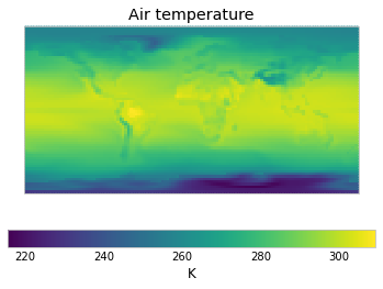
We can also take a time average and make a spatial plot.

[13]:

# NBVAL_IGNORE_OUTPUT
time_mean = tas.cube.collapsed("time", iris.analysis.MEAN)
qplt.pcolormesh(time_mean);

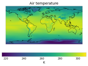
Add a spatial plot with coastlines.

[14]:

# NBVAL_IGNORE_OUTPUT
# we ignore output here as CI sometimes has to
# download the map file
qplt.pcolormesh(time_mean,)
plt.gca().coastlines();

SCM specifics¶

Finally, we present the key functions of this package. These are directly related to processing netCDF files for simple climate models.

Getting SCM timeseries¶

The major one is get_scm_timeseries. This function wraps a number of steps:

load the land surface fraction data
combine the land surface fraction and latitude data to determine the hemisphere and land/ocean boxes
cut the data into the relevant boxes
take a time average in each box
return it all as an ScmRun instance

As you can imagine, we find it very useful to be able to abstract all these normally nasty steps away.

[15]:

tas_scm_timeseries = tas.get_scm_timeseries()
type(tas_scm_timeseries)

[15]:

scmdata.run.ScmRun

[16]:

tas_scm_timeseries.tail()

[16]:

									time	1892-01-16 12:00:00	1892-02-15 00:00:00	1892-03-16 12:00:00	1892-04-16 00:00:00	1892-05-16 12:00:00	1892-06-16 00:00:00	1892-07-16 12:00:00	1892-08-16 12:00:00	1892-09-16 00:00:00	1892-10-16 12:00:00	...	1903-03-16 12:00:00	1903-04-16 00:00:00	1903-05-16 12:00:00	1903-06-16 00:00:00	1903-07-16 12:00:00	1903-08-16 12:00:00	1903-09-16 00:00:00	1903-10-16 12:00:00	1903-11-16 00:00:00	1903-12-16 12:00:00
activity_id	climate_model	member_id	mip_era	model	region	scenario	unit	variable	variable_standard_name
cmip5	CanESM2	r1i1p1	CMIP5	unspecified	World\|Southern Hemisphere	1pctCO2	K	tas	air_temperature	289.995973	290.172797	289.714070	288.535888	286.995946	285.540528	284.223201	284.026061	284.104412	285.718940	...	289.463490	288.250221	287.143196	285.560893	284.483592	284.028544	284.407818	285.688775	287.605868	289.166832
					World\|Northern Hemisphere\|Land	1pctCO2	K	tas	air_temperature	273.761214	274.977433	279.443819	285.065822	290.592045	295.710179	298.054659	296.513476	291.840867	285.930817	...	280.092979	285.314135	290.661860	295.907703	298.376198	296.972201	292.059519	286.135415	280.426803	275.705298
					World\|Southern Hemisphere\|Land	1pctCO2	K	tas	air_temperature	285.622468	284.234503	282.236887	279.420272	277.156861	275.346434	273.870726	276.048329	276.954356	280.633229	...	281.224552	278.331160	277.761742	275.291770	274.902389	275.396653	277.198751	280.436202	283.624803	285.681420
					World\|Northern Hemisphere\|Ocean	1pctCO2	K	tas	air_temperature	289.822557	289.047582	289.343519	290.817539	292.586042	294.197028	295.573417	296.190904	295.730899	294.419906	...	289.406973	290.787364	292.588619	294.351466	295.773334	296.487474	296.136925	294.893012	293.140459	291.236986
					World\|Southern Hemisphere\|Ocean	1pctCO2	K	tas	air_temperature	291.079561	291.644080	291.566631	290.794390	289.433696	288.066236	286.788149	286.002639	285.875923	286.978986	...	291.504785	290.707786	289.467563	288.105189	286.857449	286.167197	286.193950	286.990162	288.592224	290.030384

5 rows × 144 columns

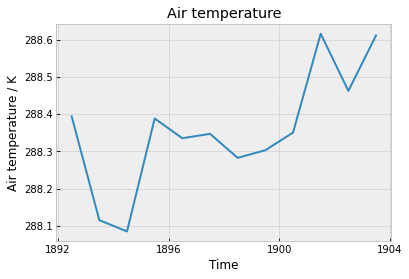
Having the data as an ScmRun makes it trivial to plot and work with.

[17]:

# NBVAL_IGNORE_OUTPUT
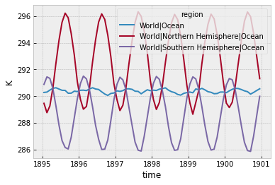
restricted_time_df = tas_scm_timeseries.filter(
    year=range(1895, 1901),
    region="*Ocean*",  # Try e.g. "*", "World", "*Land", "*Southern Hemisphere*" here
)
restricted_time_df.line_plot(
    x="time", hue="region",
);

[18]:

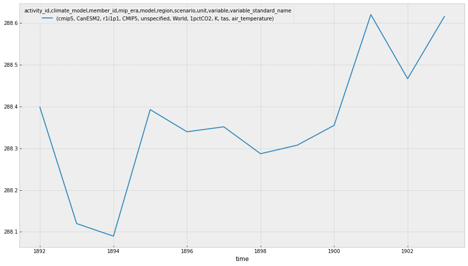
# NBVAL_IGNORE_OUTPUT
tas_scm_timeseries_annual_mean = (
    tas_scm_timeseries.filter(region="World").timeseries().T
)
tas_scm_timeseries_annual_mean = tas_scm_timeseries_annual_mean.groupby(
    tas_scm_timeseries_annual_mean.index.map(lambda x: x.year)
).mean()
tas_scm_timeseries_annual_mean.head()

[18]:

activity_id	cmip5
climate_model	CanESM2
member_id	r1i1p1
mip_era	CMIP5
model	unspecified
region	World
scenario	1pctCO2
unit	K
variable	tas
variable_standard_name	air_temperature
time
1892	288.398356
1893	288.119690
1894	288.089608
1895	288.392593
1896	288.339564

[19]:

tas_scm_timeseries_annual_mean.plot(figsize=(16, 9));

Getting SCM timeseries cubes¶

As part of the process above, we calculate all the timeseries as iris.cube.Cube’s. Extracting these intermediate cubes can be done with get_scm_timeseries_cubes. These intermediate cubes are useful as they contain all the metadata from the source cube in a slightly more friendly format than ScmRun’s metadata attribute [Note: ScmRun’s metadata handling is a work in progress].

[20]:

tas_scm_ts_cubes = tas.get_scm_timeseries_cubes()

[21]:

# NBVAL_IGNORE_OUTPUT
print(tas_scm_ts_cubes["World"].cube)

air_temperature                               (time: 144)
     Dimension coordinates:
          time                                     x
     Scalar coordinates:
          area_world: 510099672793088.0 m**2
          area_world_land: 154606610000000.0 m**2
          area_world_northern_hemisphere: 255049836396544.0 m**2
          area_world_northern_hemisphere_land: 103962633261056.0 m**2
          area_world_northern_hemisphere_ocean: 151087203135488.0 m**2
          area_world_ocean: 355493070000000.0 m**2
          area_world_southern_hemisphere: 255049836396544.0 m**2
          area_world_southern_hemisphere_land: 50643977650176.0 m**2
          area_world_southern_hemisphere_ocean: 204405858746368.0 m**2
          height: 2.0 m
          land_fraction: 0.30309097827134884
          land_fraction_northern_hemisphere: 0.4076169376537766
          land_fraction_southern_hemisphere: 0.19856502699902237
          latitude: 0.0 degrees, bound=(-90.0, 90.0) degrees
          longitude: 178.59375 degrees, bound=(-1.40625, 358.59375) degrees
    Scalar cell measures:
          cell_area
     Attributes:
          CCCma_data_licence: 1) GRANT OF LICENCE - The Government of Canada (Environment Canada) is...
          CCCma_parent_runid: IGA
          CCCma_runid: IDK
          CDI: Climate Data Interface version 1.9.7.1 (http://mpimet.mpg.de/cdi)
          CDO: Climate Data Operators version 1.9.7.1 (http://mpimet.mpg.de/cdo)
          Conventions: CF-1.4
          activity_id: cmip5
          associated_files: baseURL: http://cmip-pcmdi.llnl.gov/CMIP5/dataLocation gridspecFile: gridspec_atmos_fx_CanESM2_1pctCO2_r0i0p0.nc...
          branch_time: 171915.0
          branch_time_YMDH: 2321:01:01:00
          climate_model: CanESM2
          cmor_version: 2.5.4
          contact: cccma_info@ec.gc.ca
          creation_date: 2011-03-10T12:09:13Z
          crunch_netcdf_scm_version: 2.0.0rc5+3.gc7d2d42.dirty (more info at gitlab.com/netcdf-scm/netcdf-s...
          crunch_netcdf_scm_weight_kwargs: {}
          crunch_source_files: Files: ['/cmip5/1pctCO2/Amon/tas/CanESM2/r1i1p1/tas_Amon_CanESM2_1pctCO2_r1i1p1_189201-190312.nc'];...
          experiment: 1 percent per year CO2
          experiment_id: 1pctCO2
          forcing: GHG (GHG includes CO2 only)
          frequency: mon
          history: 2011-03-10T12:09:13Z altered by CMOR: Treated scalar dimension: 'height'....
          initialization_method: 1
          institute_id: CCCma
          institution: CCCma (Canadian Centre for Climate Modelling and Analysis, Victoria, BC,...
          member_id: r1i1p1
          mip_era: CMIP5
          model_id: CanESM2
          modeling_realm: atmos
          original_name: ST
          parent_experiment: pre-industrial control
          parent_experiment_id: piControl
          parent_experiment_rip: r1i1p1
          physics_version: 1
          product: output
          project_id: CMIP5
          realization: 1
          references: http://www.cccma.ec.gc.ca/models
          region: World
          scenario: 1pctCO2
          source: CanESM2 2010 atmosphere: CanAM4 (AGCM15i, T63L35) ocean: CanOM4 (OGCM4.0,...
          table_id: Table Amon (31 January 2011) 53b766a395ac41696af40aab76a49ae5
          title: CanESM2 model output prepared for CMIP5 1 percent per year CO2
          tracking_id: 36b6de63-cce5-4a7a-a3f4-69e5b4056fde
          variable: tas
          variable_standard_name: air_temperature
     Cell methods:
          mean: time (15 minutes)
          mean: latitude, longitude

In particular, the land_fraction* auxillary co-ordinates provide useful information about the fraction of area that was assumed to be land in the crunching.

[22]:

tas_scm_ts_cubes["World"].cube.coords("land_fraction")

[22]:

[AuxCoord(array([0.30309098]), standard_name=None, units=Unit('1'), long_name='land_fraction')]

[23]:

tas_scm_ts_cubes["World"].cube.coords("land_fraction_northern_hemisphere")

[23]:

[AuxCoord(array([0.40761694]), standard_name=None, units=Unit('1'), long_name='land_fraction_northern_hemisphere')]

Investigating the weights¶

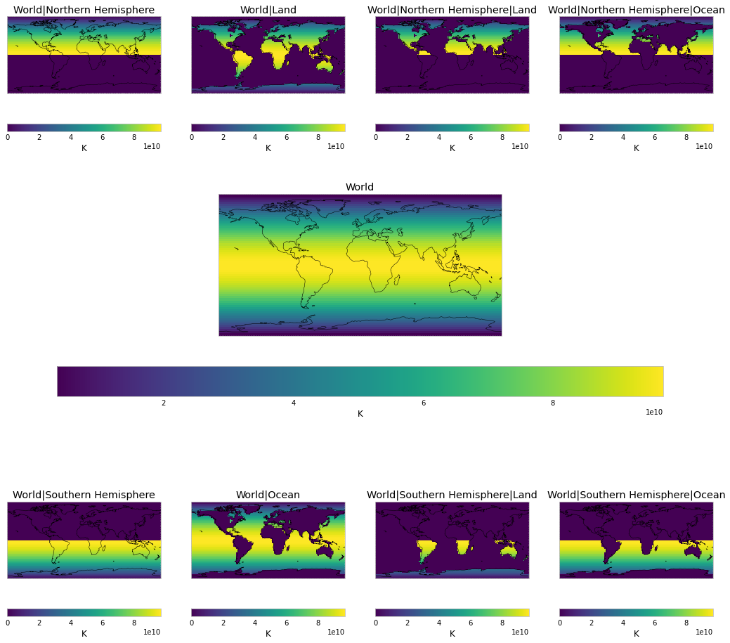
Another utility function is get_scm_timeseries_weights. This function is very similar to get_scm_timeseries but returns just the weights rather than a ScmRun. These weights are also area weighted.

[24]:

tas_scm_weights = tas.get_scm_timeseries_weights()

[25]:

# NBVAL_IGNORE_OUTPUT
plt.figure(figsize=(18, 18))
no_rows = 3
no_cols = 4

total_panels = no_cols * no_rows
rows_plt_comp = no_rows * 100
cols_plt_comp = no_cols * 10
for i, (label, weights) in enumerate(tas_scm_weights.items()):
    if label == "World":
        index = int((no_rows + 1) / 2)
        plt.subplot(no_rows, 1, index)
    else:
        if label == "World|Northern Hemisphere":
            index = 1
        elif label == "World|Southern Hemisphere":
            index = 1 + (no_rows - 1) * no_cols
        elif label == "World|Land":
            index = 2
        elif label == "World|Ocean":
            index = 2 + (no_rows - 1) * no_cols
        else:
            index = 3
            if "Ocean" in label:
                index += 1
            if "Southern Hemisphere" in label:
                index += (no_rows - 1) * no_cols

        plt.subplot(no_rows, no_cols, index)

    weight_cube = tas.cube.collapsed("time", iris.analysis.MEAN)
    weight_cube.data = weights
    qplt.pcolormesh(weight_cube)
    plt.title(label)
    plt.gca().coastlines()


plt.tight_layout()

<ipython-input-25-462c0f3bdde1>:38: UserWarning: Tight layout not applied. tight_layout cannot make axes width small enough to accommodate all axes decorations
  plt.tight_layout()