Stitching and Normalisation
In this notebook we look at how to stitch CMIP6 output files together to create continuous timeseries and how to determine how to normalise these files e.g. calculate anomalies against piControl runs.
[1]:
# NBVAL_IGNORE_OUTPUT
import datetime as dt
import glob
import os.path
from pathlib import Path

import matplotlib
import matplotlib.pyplot as plt
import pymagicc
import seaborn as sns
import tqdm
from scmdata import run_append, ScmRun

from netcdf_scm.io import load_mag_file, load_scmrun
from netcdf_scm.normalisation import get_normaliser
from netcdf_scm.stitching import (
    get_branch_time,
    get_parent_file_path,
    get_parent_replacements,
    step_up_family_tree,
)
[2]:
plt.style.use("bmh")
%matplotlib inline
Command line interface help
The help can be accessed via our command line interface.
[3]:
# NBVAL_IGNORE_OUTPUT
!netcdf-scm stitch -h
Usage: netcdf-scm stitch [OPTIONS] SRC DST STITCH_CONTACT

  Stitch netCDF-SCM ``.nc`` files together and write out in the specified
  format.

  ``SRC`` is searched recursively and netcdf-scm will attempt to stitch all
  the files found. Output is written in ``DST``.

  ``STITCH_CONTACT`` is written into the header of the output files.

Options:
  --regexp TEXT                   Regular expression to apply to file
                                  directory (only stitches matches). Be
                                  careful, if you use a very copmlex regexp
                                  directory sorting can be extremely slow (see
                                  e.g. discussion at
                                  https://stackoverflow.com/a/5428712)!
                                  [default: ^(?!.*(fx)).*$]

  --prefix TEXT                   Prefix to apply to output file names (not
                                  paths).

  --out-format [mag-files|mag-files-average-year-start-year|mag-files-average-year-mid-year|mag-files-average-year-end-year|mag-files-point-start-year|mag-files-point-mid-year|mag-files-point-end-year|magicc-input-files|magicc-input-files-average-year-start-year|magicc-input-files-average-year-mid-year|magicc-input-files-average-year-end-year|magicc-input-files-point-start-year|magicc-input-files-point-mid-year|magicc-input-files-point-end-year|tuningstrucs-blend-model]
                                  Format to re-write crunched data into. The
                                  time operation conventions follow those in
                                  `Pymagicc <https://pymagicc.readthedocs.io/e
                                  n/latest/file_conventions.html#namelists>`_
                                  .  [default: mag-files]

  --drs [None|MarbleCMIP5|CMIP6Input4MIPs|CMIP6Output]
                                  Data reference syntax to use to decipher
                                  paths. This is required to ensure the output
                                  folders match the input data reference
                                  syntax.  [default: None]

  -f, --force / --do-not-force    Overwrite any existing files.  [default:
                                  False]

  --number-workers INTEGER        Number of worker (threads) to use when
                                  stitching.  [default: 4]

  --target-units-specs PATH       csv containing target units for stitched
                                  variables.

  --normalise [31-yr-mean-after-branch-time|21-yr-running-mean|21-yr-running-mean-dedrift|30-yr-running-mean|30-yr-running-mean-dedrift]
                                  How to normalise the data relative to
                                  piControl (if not provided, no normalisation
                                  is performed).

  -h, --help                      Show this message and exit.
Stitching
Stitching simply refers to joining a child scenario with its parent. For example, an ssp with its corresponding historical run.
[4]:
# NBVAL_IGNORE_OUTPUT
!netcdf-scm stitch \
    "../../../tests/test-data/expected-crunching-output/cmip6output" \
    "../../../output-examples/stitched-files" \
    "notebook example <email address>" \
    --force \
    --drs "CMIP6Output" \
    --regexp ".*EC-Earth3-Veg.*ssp585.*r1i1p1f1.*hfds.*"
23524 2020-10-08 13:09:03,196 INFO:netcdf_scm:netcdf-scm: 2.0.0rc5+9.gf0c1d5a.dirty
23524 2020-10-08 13:09:03,196 INFO:netcdf_scm:stitch-contact: notebook example <email address>
23524 2020-10-08 13:09:03,196 INFO:netcdf_scm:source: /Users/znicholls/Documents/AGCEC/netCDF-SCM/netcdf-scm/tests/test-data/expected-crunching-output/cmip6output
23524 2020-10-08 13:09:03,196 INFO:netcdf_scm:destination: /Users/znicholls/Documents/AGCEC/netCDF-SCM/netcdf-scm/output-examples/stitched-files
23524 2020-10-08 13:09:03,196 INFO:netcdf_scm:regexp: .*EC-Earth3-Veg.*ssp585.*r1i1p1f1.*hfds.*
23524 2020-10-08 13:09:03,197 INFO:netcdf_scm:prefix: None
23524 2020-10-08 13:09:03,197 INFO:netcdf_scm:out-format: mag-files
23524 2020-10-08 13:09:03,197 INFO:netcdf_scm:drs: CMIP6Output
23524 2020-10-08 13:09:03,197 INFO:netcdf_scm:force: True
23524 2020-10-08 13:09:03,197 INFO:netcdf_scm:number-workers: 4
23524 2020-10-08 13:09:03,197 INFO:netcdf_scm:target-units-specs: None
23524 2020-10-08 13:09:03,197 INFO:netcdf_scm:normalise: None
23524 2020-10-08 13:09:03,197 INFO:netcdf_scm:Finding directories with files
Walking through directories and applying `check_func`: 337it [00:00, 19754.04it/s]
23524 2020-10-08 13:09:03,221 INFO:netcdf_scm:Found 1 directories with files
23524 2020-10-08 13:09:03,221 INFO:netcdf_scm.cli_parallel:Processing in parallel with 4 workers
23524 2020-10-08 13:09:03,221 INFO:netcdf_scm.cli_parallel:Forcing dask to use a single thread when reading
100%|████████████████████████████████████████| 1.00/1.00 [00:08<00:00, 8.66s/it]
We can then load the resulting files.
[5]:
written_files = [
    f
    for f in Path("../../../output-examples/stitched-files/CMIP6").rglob(
        "*.MAG"
    )
]
written_files
[5]:
[PosixPath('../../../output-examples/stitched-files/CMIP6/ScenarioMIP/EC-Earth-Consortium/EC-Earth3-Veg/ssp585/r1i1p1f1/Omon/hfds/gn/v20190629/netcdf-scm_hfds_Omon_EC-Earth3-Veg_ssp585_r1i1p1f1_gn_201201-201712.MAG')]
As we can see below, the output file is the result of joining the scenario and historical file (i.e. we have data pre-2015, which is when the scenario started).
[6]:
# NBVAL_IGNORE_OUTPUT
stitched = load_mag_file(str(written_files[0]), drs="CMIP6Output")
stitched.timeseries()
[6]:
| time | 2012-01-15 12:00:00 | 2012-02-14 12:00:00 | 2012-03-15 12:00:00 | 2012-04-15 00:00:00 | 2012-05-15 12:00:00 | 2012-06-15 00:00:00 | 2012-07-15 12:00:00 | 2012-08-15 12:00:00 | 2012-09-15 00:00:00 | 2012-10-15 12:00:00 | ... | 2017-03-15 12:00:00 | 2017-04-15 00:00:00 | 2017-05-15 12:00:00 | 2017-06-15 00:00:00 | 2017-07-15 12:00:00 | 2017-08-15 12:00:00 | 2017-09-15 00:00:00 | 2017-10-15 12:00:00 | 2017-11-15 00:00:00 | 2017-12-15 12:00:00 | ||||||||
|---|---|---|---|---|---|---|---|---|---|---|---|---|---|---|---|---|---|---|---|---|---|---|---|---|---|---|---|---|---|
| activity_id | climate_model | member_id | mip_era | model | region | scenario | unit | variable | |||||||||||||||||||||
| ScenarioMIP | EC-Earth3-Veg | r1i1p1f1 | CMIP6 | unspecified | World | ssp585 | W m^-2 | hfds | 6.09994 | 2.72503 | -0.248865 | -9.44095 | -18.7506 | -22.8179 | -22.7796 | -12.2644 | 1.86888 | 12.4186 | ... | -2.99801 | -8.95005 | -19.2735 | -23.6987 | -20.5724 | -10.7912 | 0.277462 | 9.32262 | 12.4736 | 4.49684 |
| World|El Nino N3.4 | ssp585 | W m^-2 | hfds | 42.06670 | 60.51390 | 64.278200 | 71.26870 | 47.5103 | 41.5238 | 31.4823 | 58.7500 | 68.34040 | 59.2635 | ... | 12.78220 | 23.66410 | 21.0705 | 16.0603 | 24.3034 | 55.1825 | 69.165500 | 72.93310 | 68.8009 | 48.85080 | |||||
| World|North Atlantic Ocean | ssp585 | W m^-2 | hfds | -131.94000 | -72.55420 | -26.789700 | 5.30091 | 70.4493 | 90.9213 | 85.4514 | 62.1627 | 13.67660 | -34.1867 | ... | -27.64220 | 19.14390 | 80.5870 | 87.5091 | 83.8828 | 55.5308 | 23.421100 | -49.07170 | -105.0520 | -126.40200 | |||||
| World|Northern Hemisphere | ssp585 | W m^-2 | hfds | -104.36000 | -71.78500 | -16.934200 | 24.85200 | 64.1233 | 79.7790 | 73.3478 | 53.5719 | 15.74550 | -35.0989 | ... | -25.98130 | 25.94270 | 67.3027 | 78.7684 | 73.2868 | 56.7929 | 14.830600 | -35.79080 | -85.7740 | -115.50600 | |||||
| World|Northern Hemisphere|Ocean | ssp585 | W m^-2 | hfds | -104.36000 | -71.78500 | -16.934200 | 24.85200 | 64.1233 | 79.7790 | 73.3478 | 53.5719 | 15.74550 | -35.0989 | ... | -25.98130 | 25.94270 | 67.3027 | 78.7684 | 73.2868 | 56.7929 | 14.830600 | -35.79080 | -85.7740 | -115.50600 | |||||
| World|Ocean | ssp585 | W m^-2 | hfds | 6.09994 | 2.72503 | -0.248865 | -9.44095 | -18.7506 | -22.8179 | -22.7796 | -12.2644 | 1.86888 | 12.4186 | ... | -2.99801 | -8.95005 | -19.2735 | -23.6987 | -20.5724 | -10.7912 | 0.277462 | 9.32262 | 12.4736 | 4.49684 | |||||
| World|Southern Hemisphere | ssp585 | W m^-2 | hfds | 93.36680 | 61.59030 | 12.933100 | -36.53350 | -84.2235 | -103.8730 | -98.7233 | -64.2772 | -9.09406 | 49.9590 | ... | 15.15950 | -36.51640 | -87.6713 | -104.6510 | -94.7240 | -64.1846 | -11.220000 | 44.96360 | 90.0923 | 99.30250 | |||||
| World|Southern Hemisphere|Ocean | ssp585 | W m^-2 | hfds | 93.36680 | 61.59030 | 12.933100 | -36.53350 | -84.2235 | -103.8730 | -98.7233 | -64.2772 | -9.09406 | 49.9590 | ... | 15.15950 | -36.51640 | -87.6713 | -104.6510 | -94.7240 | -64.1846 | -11.220000 | 44.96360 | 90.0923 | 99.30250 |
8 rows × 72 columns
[7]:
# NBVAL_IGNORE_OUTPUT
ax = plt.figure(figsize=(12, 8)).add_subplot(111)
stitched.lineplot(hue="region", ax=ax)
[7]:
<AxesSubplot:xlabel='time', ylabel='W m^-2'>
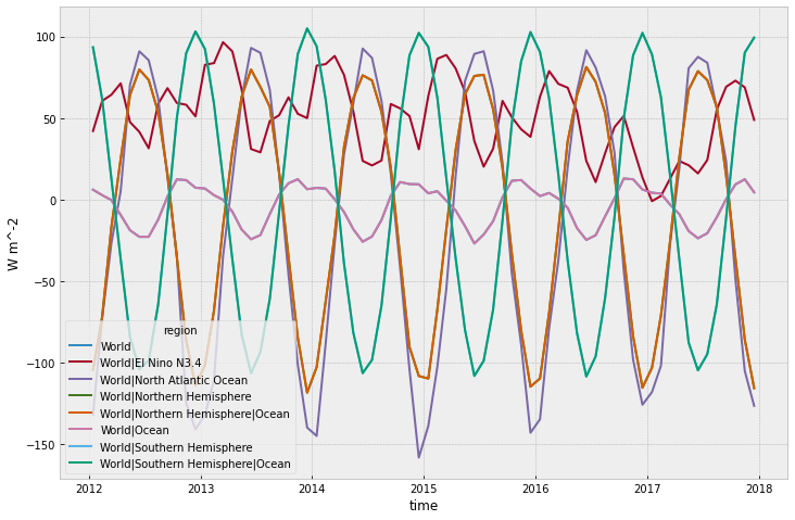
The files are also written with extensive metadata, which we can access via the MAGICCData instance’s .metadata attribute. The ‘child’ metadata is the metadata of the ‘child’ simulation (in this case ‘ssp585’) while the parent data is the data from the simulation the ‘child’ branched off (in this case ‘historical’).
[8]:
# NBVAL_IGNORE_OUTPUT
stitched.metadata
[8]:
{'timeseriestype': 'MONTHLY',
 'date': '2020-10-08 13:09:11',
 'contact': 'notebook example <email address>',
 '(child) CDI': 'Climate Data Interface version 1.8.2 (http://mpimet.mpg.de/cdi)',
 '(child) CDO': 'Climate Data Operators version 1.8.2 (http://mpimet.mpg.de/cdo)',
 '(child) Conventions': 'CF-1.7',
 '(child) area_world (m**2)': '510045092655104.0',
 '(child) area_world_el_nino_n3.4 (m**2)': '6657359020032.0',
 '(child) area_world_north_atlantic_ocean (m**2)': '55474658279424.0',
 '(child) area_world_northern_hemisphere (m**2)': '225108691435520.0',
 '(child) area_world_northern_hemisphere_ocean (m**2)': '225108691435520.0',
 '(child) area_world_ocean (m**2)': '510045092655104.0',
 '(child) area_world_southern_hemisphere (m**2)': '284936401219584.0',
 '(child) area_world_southern_hemisphere_ocean (m**2)': '284936401219584.0',
 '(child) branch_method': 'standard',
 '(child) branch_time_in_child': '60265.0',
 '(child) branch_time_in_parent': '60265.0',
 '(child) calendar': 'proleptic_gregorian',
 '(child) cmor_version': '3.4.0',
 '(child) comment': "This is the net flux of heat entering the liquid water column through its upper surface (excluding any 'flux adjustment') .",
 '(child) contact': 'cmip6-data@ec-earth.org',
 '(child) crunch_contact': 'cmip6output crunching regression test',
 '(child) crunch_netcdf_scm_version': '2.0.0rc2+96.gbb78b86.dirty (more info at gitlab.com/netcdf-scm/netcdf-scm)',
 '(child) crunch_netcdf_scm_weight_kwargs': '{"regions": ["World", "World|Northern Hemisphere", "World|Southern Hemisphere", "World|Ocean", "World|Northern Hemisphere|Ocean", "World|Southern Hemisphere|Ocean", "World|North Atlantic Ocean", "World|El Nino N3.4"], "cell_weights": null}',
 '(child) crunch_source_files': "Files: ['/CMIP6/ScenarioMIP/EC-Earth-Consortium/EC-Earth3-Veg/ssp585/r1i1p1f1/Omon/hfds/gn/v20190629/hfds_Omon_EC-Earth3-Veg_ssp585_r1i1p1f1_gn_201501-201512.nc', '/CMIP6/ScenarioMIP/EC-Earth-Consortium/EC-Earth3-Veg/ssp585/r1i1p1f1/Omon/hfds/gn/v20190629/hfds_Omon_EC-Earth3-Veg_ssp585_r1i1p1f1_gn_201601-201612.nc', '/CMIP6/ScenarioMIP/EC-Earth-Consortium/EC-Earth3-Veg/ssp585/r1i1p1f1/Omon/hfds/gn/v20190629/hfds_Omon_EC-Earth3-Veg_ssp585_r1i1p1f1_gn_201701-201712.nc']; areacello: ['/CMIP6/ScenarioMIP/EC-Earth-Consortium/EC-Earth3-Veg/ssp585/r1i1p1f1/Ofx/areacello/gn/v20190629/areacello_Ofx_EC-Earth3-Veg_ssp585_r1i1p1f1_gn.nc']",
 '(child) data_specs_version': '01.00.30',
 '(child) experiment': 'update of RCP8.5 based on SSP5',
 '(child) experiment_id': 'ssp585',
 '(child) external_variables': 'areacello',
 '(child) forcing_index': '1',
 '(child) frequency': 'mon',
 '(child) further_info_url': 'https://furtherinfo.es-doc.org/CMIP6.EC-Earth-Consortium.EC-Earth3-Veg.ssp585.none.r1i1p1f1',
 '(child) grid': 'T255L91-ORCA1L75',
 '(child) grid_label': 'gn',
 '(child) initialization_index': '1',
 '(child) institution': 'AEMET, Spain; BSC, Spain; CNR-ISAC, Italy; DMI, Denmark; ENEA, Italy; FMI, Finland; Geomar, Germany; ICHEC, Ireland; ICTP, Italy; IDL, Portugal; IMAU, The Netherlands; IPMA, Portugal; KIT, Karlsruhe, Germany; KNMI, The Netherlands; Lund University, Sweden; Met Eireann, Ireland; NLeSC, The Netherlands; NTNU, Norway; Oxford University, UK; surfSARA, The Netherlands; SMHI, Sweden; Stockholm University, Sweden; Unite ASTR, Belgium; University College Dublin, Ireland; University of Bergen, Norway; University of Copenhagen, Denmark; University of Helsinki, Finland; University of Santiago de Compostela, Spain; Uppsala University, Sweden; Utrecht University, The Netherlands; Vrije Universiteit Amsterdam, the Netherlands; Wageningen University, The Netherlands. Mailing address: EC-Earth consortium, Rossby Center, Swedish Meteorological and Hydrological Institute/SMHI, SE-601 76 Norrkoping, Sweden',
 '(child) institution_id': 'EC-Earth-Consortium',
 '(child) license': 'CMIP6 model data produced by EC-Earth-Consortium is licensed under a Creative Commons Attribution-ShareAlike 4.0 International License (https://creativecommons.org/licenses). Consult https://pcmdi.llnl.gov/CMIP6/TermsOfUse for terms of use governing CMIP6 output, including citation requirements and proper acknowledgment. Further information about this data, including some limitations, can be found via the further_info_url (recorded as a global attribute in this file) and at http://www.ec-earth.org. The data producers and data providers make no warranty, either express or implied, including, but not limited to, warranties of merchantability and fitness for a particular purpose. All liabilities arising from the supply of the information (including any liability arising in negligence) are excluded to the fullest extent permitted by law.',
 '(child) netcdf-scm crunched file': 'CMIP6/ScenarioMIP/EC-Earth-Consortium/EC-Earth3-Veg/ssp585/r1i1p1f1/Omon/hfds/gn/v20190629/netcdf-scm_hfds_Omon_EC-Earth3-Veg_ssp585_r1i1p1f1_gn_201501-201712.nc',
 '(child) nominal_resolution': '100 km',
 '(child) original_name': 'hfds',
 '(child) parent_activity_id': 'CMIP',
 '(child) parent_experiment_id': 'historical',
 '(child) parent_mip_era': 'CMIP6',
 '(child) parent_source_id': 'EC-Earth3-Veg',
 '(child) parent_time_units': 'days since 1850-01-01',
 '(child) parent_variant_label': 'r1i1p1f1',
 '(child) physics_index': '1',
 '(child) product': 'model-output',
 '(child) realization_index': '1',
 '(child) realm': 'ocean',
 '(child) source': 'EC-Earth3-Veg (2019):',
 'aerosol': 'none',
 'atmos': 'IFS cy36r4 (TL255, linearly reduced Gaussian grid equivalent to 512 x 256 longitude/latitude; 91 levels; top level 0.01 hPa)',
 'atmosChem': 'none',
 'land': 'HTESSEL (land surface scheme built in IFS) and LPJ-GUESS v4',
 'landIce': 'none',
 'ocean': 'NEMO3.6 (ORCA1 tripolar primarily 1 degree with meridional refinement down to 1/3 degree in the tropics; 362 x 292 longitude/latitude; 75 levels; top grid cell 0-1 m)',
 'ocnBgchem': 'none',
 'seaIce': 'LIM3',
 '(child) source_id': 'EC-Earth3-Veg',
 '(child) source_type': 'AOGCM',
 '(child) sub_experiment': 'none',
 '(child) sub_experiment_id': 'none',
 '(child) table_id': 'Omon',
 '(child) table_info': 'Creation Date:(09 May 2019) MD5:cde930676e68ac6780d5e4c62d3898f6',
 '(child) title': 'EC-Earth3-Veg output prepared for CMIP6',
 '(child) variable_id': 'hfds',
 '(child) variant_label': 'r1i1p1f1',
 '(parent) CDI': 'Climate Data Interface version 1.8.2 (http://mpimet.mpg.de/cdi)',
 '(parent) CDO': 'Climate Data Operators version 1.8.2 (http://mpimet.mpg.de/cdo)',
 '(parent) Conventions': 'CF-1.7',
 '(parent) area_world (m**2)': '510045092655104.0',
 '(parent) area_world_el_nino_n3.4 (m**2)': '6657359020032.0',
 '(parent) area_world_north_atlantic_ocean (m**2)': '55474658279424.0',
 '(parent) area_world_northern_hemisphere (m**2)': '225108691435520.0',
 '(parent) area_world_northern_hemisphere_ocean (m**2)': '225108691435520.0',
 '(parent) area_world_ocean (m**2)': '510045092655104.0',
 '(parent) area_world_southern_hemisphere (m**2)': '284936401219584.0',
 '(parent) area_world_southern_hemisphere_ocean (m**2)': '284936401219584.0',
 '(parent) branch_method': 'standard',
 '(parent) branch_time_in_child': '0.0',
 '(parent) branch_time_in_parent': '65744.0',
 '(parent) calendar': 'gregorian',
 '(parent) cmor_version': '3.4.0',
 '(parent) comment': "This is the net flux of heat entering the liquid water column through its upper surface (excluding any 'flux adjustment') .",
 '(parent) contact': 'cmip6-data@ec-earth.org',
 '(parent) crunch_contact': 'cmip6output crunching regression test',
 '(parent) crunch_netcdf_scm_version': '2.0.0rc2+96.gbb78b86.dirty (more info at gitlab.com/netcdf-scm/netcdf-scm)',
 '(parent) crunch_netcdf_scm_weight_kwargs': '{"regions": ["World", "World|Northern Hemisphere", "World|Southern Hemisphere", "World|Ocean", "World|Northern Hemisphere|Ocean", "World|Southern Hemisphere|Ocean", "World|North Atlantic Ocean", "World|El Nino N3.4"], "cell_weights": null}',
 '(parent) crunch_source_files': "Files: ['/CMIP6/CMIP/EC-Earth-Consortium/EC-Earth3-Veg/historical/r1i1p1f1/Omon/hfds/gn/v20190605/hfds_Omon_EC-Earth3-Veg_historical_r1i1p1f1_gn_201201-201212.nc', '/CMIP6/CMIP/EC-Earth-Consortium/EC-Earth3-Veg/historical/r1i1p1f1/Omon/hfds/gn/v20190605/hfds_Omon_EC-Earth3-Veg_historical_r1i1p1f1_gn_201301-201312.nc', '/CMIP6/CMIP/EC-Earth-Consortium/EC-Earth3-Veg/historical/r1i1p1f1/Omon/hfds/gn/v20190605/hfds_Omon_EC-Earth3-Veg_historical_r1i1p1f1_gn_201401-201412.nc']; areacello: ['/CMIP6/CMIP/EC-Earth-Consortium/EC-Earth3-Veg/historical/r1i1p1f1/Ofx/areacello/gn/v20190605/areacello_Ofx_EC-Earth3-Veg_historical_r1i1p1f1_gn.nc']",
 '(parent) data_specs_version': '01.00.30',
 '(parent) experiment': 'all-forcing simulation of the recent past',
 '(parent) experiment_id': 'historical',
 '(parent) external_variables': 'areacello',
 '(parent) forcing_index': '1',
 '(parent) frequency': 'mon',
 '(parent) further_info_url': 'https://furtherinfo.es-doc.org/CMIP6.EC-Earth-Consortium.EC-Earth3-Veg.historical.none.r1i1p1f1',
 '(parent) grid': 'T255L91-ORCA1L75',
 '(parent) grid_label': 'gn',
 '(parent) initialization_index': '1',
 '(parent) institution': 'AEMET, Spain; BSC, Spain; CNR-ISAC, Italy; DMI, Denmark; ENEA, Italy; FMI, Finland; Geomar, Germany; ICHEC, Ireland; ICTP, Italy; IDL, Portugal; IMAU, The Netherlands; IPMA, Portugal; KIT, Karlsruhe, Germany; KNMI, The Netherlands; Lund University, Sweden; Met Eireann, Ireland; NLeSC, The Netherlands; NTNU, Norway; Oxford University, UK; surfSARA, The Netherlands; SMHI, Sweden; Stockholm University, Sweden; Unite ASTR, Belgium; University College Dublin, Ireland; University of Bergen, Norway; University of Copenhagen, Denmark; University of Helsinki, Finland; University of Santiago de Compostela, Spain; Uppsala University, Sweden; Utrecht University, The Netherlands; Vrije Universiteit Amsterdam, the Netherlands; Wageningen University, The Netherlands. Mailing address: EC-Earth consortium, Rossby Center, Swedish Meteorological and Hydrological Institute/SMHI, SE-601 76 Norrkoping, Sweden',
 '(parent) institution_id': 'EC-Earth-Consortium',
 '(parent) license': 'CMIP6 model data produced by EC-Earth-Consortium is licensed under a Creative Commons Attribution-ShareAlike 4.0 International License (https://creativecommons.org/licenses). Consult https://pcmdi.llnl.gov/CMIP6/TermsOfUse for terms of use governing CMIP6 output, including citation requirements and proper acknowledgment. Further information about this data, including some limitations, can be found via the further_info_url (recorded as a global attribute in this file) and at http://www.ec-earth.org. The data producers and data providers make no warranty, either express or implied, including, but not limited to, warranties of merchantability and fitness for a particular purpose. All liabilities arising from the supply of the information (including any liability arising in negligence) are excluded to the fullest extent permitted by law.',
 '(parent) netcdf-scm crunched file': 'CMIP6/CMIP/EC-Earth-Consortium/EC-Earth3-Veg/historical/r1i1p1f1/Omon/hfds/gn/v20190605/netcdf-scm_hfds_Omon_EC-Earth3-Veg_historical_r1i1p1f1_gn_201201-201412.nc',
 '(parent) nominal_resolution': '100 km',
 '(parent) original_name': 'hfds',
 '(parent) parent_activity_id': 'CMIP',
 '(parent) parent_experiment_id': 'piControl',
 '(parent) parent_mip_era': 'CMIP6',
 '(parent) parent_source_id': 'EC-Earth3-Veg',
 '(parent) parent_time_units': 'days since 1850-01-01',
 '(parent) parent_variant_label': 'r1i1p1f1',
 '(parent) physics_index': '1',
 '(parent) product': 'model-output',
 '(parent) realization_index': '1',
 '(parent) realm': 'ocean',
 '(parent) source': 'EC-Earth3-Veg (2019):',
 '(parent) source_id': 'EC-Earth3-Veg',
 '(parent) source_type': 'AOGCM',
 '(parent) sub_experiment': 'none',
 '(parent) sub_experiment_id': 'none',
 '(parent) table_id': 'Omon',
 '(parent) table_info': 'Creation Date:(09 May 2019) MD5:cde930676e68ac6780d5e4c62d3898f6',
 '(parent) title': 'EC-Earth3-Veg output prepared for CMIP6',
 '(parent) variable_id': 'hfds',
 '(parent) variant_label': 'r1i1p1f1',
 'header': 'Source data crunched with: netCDF-SCM v2.0.0rc2+96.gbb78b86.dirty (more info at gitlab.com/netcdf-scm/netcdf-scm)\nFile written with: pymagicc v2.0.0rc6 (more info at github.com/openclimatedata/pymagicc)'}
Stitching and normalising
On top of stitching, we might also normalise. This means we find the piControl run, and then normalise our output data against the piControl somehow. The available methods shown in the help of --normalise option of netcdf-scm stitch.
[9]:
# NBVAL_IGNORE_OUTPUT
!netcdf-scm stitch --help | grep -2 normalise
                                  variables.

  --normalise [31-yr-mean-after-branch-time|21-yr-running-mean|21-yr-running-mean-dedrift|30-yr-running-mean|30-yr-running-mean-dedrift]
                                  How to normalise the data relative to
                                  piControl (if not provided, no normalisation
                                  is performed).
We can run the stitching for these five different options as shown below.
[10]:
# NBVAL_IGNORE_OUTPUT
!netcdf-scm stitch \
    "../../../tests/test-data/expected-crunching-output/marble-cmip5" \
    "../../../output-examples/stitched-normalised-files-31-yr-mean-after-branch-time" \
    "notebook example <email address>" \
    --force \
    --drs "MarbleCMIP5" \
    --regexp ".*rcp45.*tas.*NorESM1.*" \
    --normalise "31-yr-mean-after-branch-time"

!netcdf-scm stitch \
    "../../../tests/test-data/expected-crunching-output/marble-cmip5" \
    "../../../output-examples/stitched-normalised-files-21-yr-running-mean" \
    "notebook example <email address>" \
    --force \
    --drs "MarbleCMIP5" \
    --regexp ".*rcp45.*tas.*NorESM1.*" \
    --normalise "21-yr-running-mean"

!netcdf-scm stitch \
    "../../../tests/test-data/expected-crunching-output/marble-cmip5" \
    "../../../output-examples/stitched-normalised-files-21-yr-running-mean-dedrift" \
    "notebook example <email address>" \
    --force \
    --drs "MarbleCMIP5" \
    --regexp ".*rcp45.*tas.*NorESM1.*" \
    --normalise "21-yr-running-mean-dedrift"

!netcdf-scm stitch \
    "../../../tests/test-data/expected-crunching-output/marble-cmip5" \
    "../../../output-examples/stitched-normalised-files-30-yr-running-mean" \
    "notebook example <email address>" \
    --force \
    --drs "MarbleCMIP5" \
    --regexp ".*rcp45.*tas.*NorESM1.*" \
    --normalise "30-yr-running-mean"

!netcdf-scm stitch \
    "../../../tests/test-data/expected-crunching-output/marble-cmip5" \
    "../../../output-examples/stitched-normalised-files-30-yr-running-mean-dedrift" \
    "notebook example <email address>" \
    --force \
    --drs "MarbleCMIP5" \
    --regexp ".*rcp45.*tas.*NorESM1.*" \
    --normalise "30-yr-running-mean-dedrift"
23553 2020-10-08 13:09:19,549 INFO:netcdf_scm:netcdf-scm: 2.0.0rc5+9.gf0c1d5a.dirty
23553 2020-10-08 13:09:19,550 INFO:netcdf_scm:stitch-contact: notebook example <email address>
23553 2020-10-08 13:09:19,550 INFO:netcdf_scm:source: /Users/znicholls/Documents/AGCEC/netCDF-SCM/netcdf-scm/tests/test-data/expected-crunching-output/marble-cmip5
23553 2020-10-08 13:09:19,550 INFO:netcdf_scm:destination: /Users/znicholls/Documents/AGCEC/netCDF-SCM/netcdf-scm/output-examples/stitched-normalised-files-31-yr-mean-after-branch-time
23553 2020-10-08 13:09:19,550 INFO:netcdf_scm:regexp: .*rcp45.*tas.*NorESM1.*
23553 2020-10-08 13:09:19,550 INFO:netcdf_scm:prefix: None
23553 2020-10-08 13:09:19,550 INFO:netcdf_scm:out-format: mag-files
23553 2020-10-08 13:09:19,550 INFO:netcdf_scm:drs: MarbleCMIP5
23553 2020-10-08 13:09:19,550 INFO:netcdf_scm:force: True
23553 2020-10-08 13:09:19,550 INFO:netcdf_scm:number-workers: 4
23553 2020-10-08 13:09:19,550 INFO:netcdf_scm:target-units-specs: None
23553 2020-10-08 13:09:19,550 INFO:netcdf_scm:normalise: 31-yr-mean-after-branch-time
23553 2020-10-08 13:09:19,551 INFO:netcdf_scm:Finding directories with files
Walking through directories and applying `check_func`: 50it [00:00, 16016.13it/s]
23553 2020-10-08 13:09:19,561 INFO:netcdf_scm:Found 1 directories with files
23553 2020-10-08 13:09:19,561 INFO:netcdf_scm.cli_parallel:Processing in parallel with 4 workers
23553 2020-10-08 13:09:19,561 INFO:netcdf_scm.cli_parallel:Forcing dask to use a single thread when reading
100%|████████████████████████████████████████| 1.00/1.00 [00:23<00:00, 23.6s/it]
23572 2020-10-08 13:09:46,908 INFO:netcdf_scm:netcdf-scm: 2.0.0rc5+9.gf0c1d5a.dirty
23572 2020-10-08 13:09:46,908 INFO:netcdf_scm:stitch-contact: notebook example <email address>
23572 2020-10-08 13:09:46,909 INFO:netcdf_scm:source: /Users/znicholls/Documents/AGCEC/netCDF-SCM/netcdf-scm/tests/test-data/expected-crunching-output/marble-cmip5
23572 2020-10-08 13:09:46,909 INFO:netcdf_scm:destination: /Users/znicholls/Documents/AGCEC/netCDF-SCM/netcdf-scm/output-examples/stitched-normalised-files-21-yr-running-mean
23572 2020-10-08 13:09:46,909 INFO:netcdf_scm:regexp: .*rcp45.*tas.*NorESM1.*
23572 2020-10-08 13:09:46,909 INFO:netcdf_scm:prefix: None
23572 2020-10-08 13:09:46,909 INFO:netcdf_scm:out-format: mag-files
23572 2020-10-08 13:09:46,909 INFO:netcdf_scm:drs: MarbleCMIP5
23572 2020-10-08 13:09:46,909 INFO:netcdf_scm:force: True
23572 2020-10-08 13:09:46,909 INFO:netcdf_scm:number-workers: 4
23572 2020-10-08 13:09:46,909 INFO:netcdf_scm:target-units-specs: None
23572 2020-10-08 13:09:46,909 INFO:netcdf_scm:normalise: 21-yr-running-mean
23572 2020-10-08 13:09:46,909 INFO:netcdf_scm:Finding directories with files
Walking through directories and applying `check_func`: 50it [00:00, 18754.71it/s]
23572 2020-10-08 13:09:46,918 INFO:netcdf_scm:Found 1 directories with files
23572 2020-10-08 13:09:46,918 INFO:netcdf_scm.cli_parallel:Processing in parallel with 4 workers
23572 2020-10-08 13:09:46,919 INFO:netcdf_scm.cli_parallel:Forcing dask to use a single thread when reading
100%|████████████████████████████████████████| 1.00/1.00 [00:21<00:00, 21.4s/it]
23595 2020-10-08 13:10:12,480 INFO:netcdf_scm:netcdf-scm: 2.0.0rc5+9.gf0c1d5a.dirty
23595 2020-10-08 13:10:12,481 INFO:netcdf_scm:stitch-contact: notebook example <email address>
23595 2020-10-08 13:10:12,481 INFO:netcdf_scm:source: /Users/znicholls/Documents/AGCEC/netCDF-SCM/netcdf-scm/tests/test-data/expected-crunching-output/marble-cmip5
23595 2020-10-08 13:10:12,481 INFO:netcdf_scm:destination: /Users/znicholls/Documents/AGCEC/netCDF-SCM/netcdf-scm/output-examples/stitched-normalised-files-21-yr-running-mean-dedrift
23595 2020-10-08 13:10:12,481 INFO:netcdf_scm:regexp: .*rcp45.*tas.*NorESM1.*
23595 2020-10-08 13:10:12,481 INFO:netcdf_scm:prefix: None
23595 2020-10-08 13:10:12,481 INFO:netcdf_scm:out-format: mag-files
23595 2020-10-08 13:10:12,481 INFO:netcdf_scm:drs: MarbleCMIP5
23595 2020-10-08 13:10:12,481 INFO:netcdf_scm:force: True
23595 2020-10-08 13:10:12,481 INFO:netcdf_scm:number-workers: 4
23595 2020-10-08 13:10:12,481 INFO:netcdf_scm:target-units-specs: None
23595 2020-10-08 13:10:12,481 INFO:netcdf_scm:normalise: 21-yr-running-mean-dedrift
23595 2020-10-08 13:10:12,483 INFO:netcdf_scm:Finding directories with files
Walking through directories and applying `check_func`: 50it [00:00, 15995.36it/s]
23595 2020-10-08 13:10:12,493 INFO:netcdf_scm:Found 1 directories with files
23595 2020-10-08 13:10:12,494 INFO:netcdf_scm.cli_parallel:Processing in parallel with 4 workers
23595 2020-10-08 13:10:12,494 INFO:netcdf_scm.cli_parallel:Forcing dask to use a single thread when reading
100%|████████████████████████████████████████| 1.00/1.00 [00:21<00:00, 21.1s/it]
23618 2020-10-08 13:10:37,711 INFO:netcdf_scm:netcdf-scm: 2.0.0rc5+9.gf0c1d5a.dirty
23618 2020-10-08 13:10:37,712 INFO:netcdf_scm:stitch-contact: notebook example <email address>
23618 2020-10-08 13:10:37,712 INFO:netcdf_scm:source: /Users/znicholls/Documents/AGCEC/netCDF-SCM/netcdf-scm/tests/test-data/expected-crunching-output/marble-cmip5
23618 2020-10-08 13:10:37,712 INFO:netcdf_scm:destination: /Users/znicholls/Documents/AGCEC/netCDF-SCM/netcdf-scm/output-examples/stitched-normalised-files-30-yr-running-mean
23618 2020-10-08 13:10:37,712 INFO:netcdf_scm:regexp: .*rcp45.*tas.*NorESM1.*
23618 2020-10-08 13:10:37,712 INFO:netcdf_scm:prefix: None
23618 2020-10-08 13:10:37,712 INFO:netcdf_scm:out-format: mag-files
23618 2020-10-08 13:10:37,712 INFO:netcdf_scm:drs: MarbleCMIP5
23618 2020-10-08 13:10:37,712 INFO:netcdf_scm:force: True
23618 2020-10-08 13:10:37,712 INFO:netcdf_scm:number-workers: 4
23618 2020-10-08 13:10:37,712 INFO:netcdf_scm:target-units-specs: None
23618 2020-10-08 13:10:37,712 INFO:netcdf_scm:normalise: 30-yr-running-mean
23618 2020-10-08 13:10:37,712 INFO:netcdf_scm:Finding directories with files
Walking through directories and applying `check_func`: 50it [00:00, 12474.88it/s]
23618 2020-10-08 13:10:37,723 INFO:netcdf_scm:Found 1 directories with files
23618 2020-10-08 13:10:37,723 INFO:netcdf_scm.cli_parallel:Processing in parallel with 4 workers
23618 2020-10-08 13:10:37,723 INFO:netcdf_scm.cli_parallel:Forcing dask to use a single thread when reading
100%|████████████████████████████████████████| 1.00/1.00 [00:20<00:00, 20.9s/it]
23640 2020-10-08 13:11:02,583 INFO:netcdf_scm:netcdf-scm: 2.0.0rc5+9.gf0c1d5a.dirty
23640 2020-10-08 13:11:02,584 INFO:netcdf_scm:stitch-contact: notebook example <email address>
23640 2020-10-08 13:11:02,584 INFO:netcdf_scm:source: /Users/znicholls/Documents/AGCEC/netCDF-SCM/netcdf-scm/tests/test-data/expected-crunching-output/marble-cmip5
23640 2020-10-08 13:11:02,584 INFO:netcdf_scm:destination: /Users/znicholls/Documents/AGCEC/netCDF-SCM/netcdf-scm/output-examples/stitched-normalised-files-30-yr-running-mean-dedrift
23640 2020-10-08 13:11:02,584 INFO:netcdf_scm:regexp: .*rcp45.*tas.*NorESM1.*
23640 2020-10-08 13:11:02,584 INFO:netcdf_scm:prefix: None
23640 2020-10-08 13:11:02,584 INFO:netcdf_scm:out-format: mag-files
23640 2020-10-08 13:11:02,584 INFO:netcdf_scm:drs: MarbleCMIP5
23640 2020-10-08 13:11:02,584 INFO:netcdf_scm:force: True
23640 2020-10-08 13:11:02,584 INFO:netcdf_scm:number-workers: 4
23640 2020-10-08 13:11:02,584 INFO:netcdf_scm:target-units-specs: None
23640 2020-10-08 13:11:02,584 INFO:netcdf_scm:normalise: 30-yr-running-mean-dedrift
23640 2020-10-08 13:11:02,584 INFO:netcdf_scm:Finding directories with files
Walking through directories and applying `check_func`: 50it [00:00, 10586.33it/s]
23640 2020-10-08 13:11:02,596 INFO:netcdf_scm:Found 1 directories with files
23640 2020-10-08 13:11:02,597 INFO:netcdf_scm.cli_parallel:Processing in parallel with 4 workers
23640 2020-10-08 13:11:02,597 INFO:netcdf_scm.cli_parallel:Forcing dask to use a single thread when reading
100%|████████████████████████████████████████| 1.00/1.00 [00:22<00:00, 22.8s/it]
[11]:
written_files = {
    norm_id: [
        f
        for f in Path(
            "../../../output-examples/stitched-normalised-files-{}/cmip5".format(
                norm_id
            )
        ).rglob("*.MAG")
    ]
    for norm_id in [
        "31-yr-mean-after-branch-time",
        "21-yr-running-mean",
        "21-yr-running-mean-dedrift",
        "30-yr-running-mean",
        "30-yr-running-mean-dedrift",
    ]
}
written_files
[11]:
{'31-yr-mean-after-branch-time': [PosixPath('../../../output-examples/stitched-normalised-files-31-yr-mean-after-branch-time/cmip5/rcp45/Amon/tas/NorESM1-M/r1i1p1/netcdf-scm_tas_Amon_NorESM1-M_rcp45_r1i1p1_185001-230012.MAG')],
 '21-yr-running-mean': [PosixPath('../../../output-examples/stitched-normalised-files-21-yr-running-mean/cmip5/rcp45/Amon/tas/NorESM1-M/r1i1p1/netcdf-scm_tas_Amon_NorESM1-M_rcp45_r1i1p1_185001-230012.MAG')],
 '21-yr-running-mean-dedrift': [PosixPath('../../../output-examples/stitched-normalised-files-21-yr-running-mean-dedrift/cmip5/rcp45/Amon/tas/NorESM1-M/r1i1p1/netcdf-scm_tas_Amon_NorESM1-M_rcp45_r1i1p1_185001-230012.MAG')],
 '30-yr-running-mean': [PosixPath('../../../output-examples/stitched-normalised-files-30-yr-running-mean/cmip5/rcp45/Amon/tas/NorESM1-M/r1i1p1/netcdf-scm_tas_Amon_NorESM1-M_rcp45_r1i1p1_185001-230012.MAG')],
 '30-yr-running-mean-dedrift': [PosixPath('../../../output-examples/stitched-normalised-files-30-yr-running-mean-dedrift/cmip5/rcp45/Amon/tas/NorESM1-M/r1i1p1/netcdf-scm_tas_Amon_NorESM1-M_rcp45_r1i1p1_185001-230012.MAG')]}
[12]:
# NBVAL_IGNORE_OUTPUT
stitched_normalised = []
for norm_id, files in written_files.items():
    assert len(files) == 1
    out = load_mag_file(str(files[0]), drs="MarbleCMIP5")
    out["normalisation_method"] = norm_id
    stitched_normalised.append(out)

stitched_normalised = run_append(stitched_normalised)
stitched_normalised.timeseries()
[12]:
| time | 1850-01-15 12:00:00 | 1850-02-14 00:00:00 | 1850-03-15 12:00:00 | 1850-04-15 00:00:00 | 1850-05-15 12:00:00 | 1850-06-15 00:00:00 | 1850-07-15 12:00:00 | 1850-08-15 12:00:00 | 1850-09-15 00:00:00 | 1850-10-15 12:00:00 | ... | 2300-03-15 12:00:00 | 2300-04-15 00:00:00 | 2300-05-15 12:00:00 | 2300-06-15 00:00:00 | 2300-07-15 12:00:00 | 2300-08-15 12:00:00 | 2300-09-15 00:00:00 | 2300-10-15 12:00:00 | 2300-11-15 00:00:00 | 2300-12-15 12:00:00 | |||||||||
|---|---|---|---|---|---|---|---|---|---|---|---|---|---|---|---|---|---|---|---|---|---|---|---|---|---|---|---|---|---|---|
| activity_id | climate_model | member_id | mip_era | model | normalisation_method | region | scenario | unit | variable | |||||||||||||||||||||
| cmip5 | NorESM1-M | r1i1p1 | CMIP5 | unspecified | 31-yr-mean-after-branch-time | World | rcp45 | K | tas | -2.062360 | -1.695470 | -0.978669 | -0.008818 | 0.897924 | 1.439600 | 1.790620 | 1.694420 | 1.167280 | -0.055348 | ... | 1.685270 | 2.56390 | 3.288130 | 3.933980 | 4.288330 | 4.359420 | 3.731510 | 2.724840 | 1.695470 | 0.963889 |
| World|El Nino N3.4 | rcp45 | K | tas | -0.318386 | 0.159077 | 0.342337 | 0.627578 | 0.579712 | 0.752038 | 0.357578 | 0.184590 | 0.001576 | -0.059699 | ... | 2.039260 | 2.03610 | 2.417170 | 2.338170 | 2.026510 | 1.856940 | 1.662470 | 1.497680 | 1.594550 | 1.697900 | ||||||
| World|Land | rcp45 | K | tas | -6.029940 | -5.108860 | -3.036910 | -0.156864 | 2.715940 | 4.460910 | 5.842120 | 5.738900 | 3.796100 | 0.195049 | ... | 0.171098 | 3.09954 | 5.484050 | 7.538320 | 8.985430 | 9.140970 | 6.933180 | 3.690290 | 0.570492 | -1.781070 | ||||||
| World|North Atlantic Ocean | rcp45 | K | tas | -2.214140 | -2.328330 | -1.923620 | -1.064490 | -0.222693 | 0.938037 | 1.916490 | 2.497720 | 2.114200 | 1.212890 | ... | 0.478465 | 1.21837 | 2.083970 | 3.335990 | 4.360270 | 4.841550 | 4.521930 | 3.587200 | 2.283270 | 1.016070 | ||||||
| World|Northern Hemisphere | rcp45 | K | tas | -6.668830 | -5.648410 | -3.318310 | -0.332735 | 2.631710 | 4.956190 | 6.315250 | 6.042610 | 4.121100 | 0.767058 | ... | -0.325949 | 2.37494 | 5.149280 | 7.567050 | 8.982350 | 8.926500 | 7.224760 | 3.979710 | 0.752720 | -1.960780 | ||||||
| World|Northern Hemisphere|Land | rcp45 | K | tas | -11.948100 | -9.233130 | -4.682970 | 0.710767 | 5.586610 | 9.106190 | 11.225800 | 10.170100 | 6.387810 | 0.115274 | ... | -1.275390 | 3.80197 | 8.504080 | 12.514100 | 14.645900 | 13.938400 | 10.101500 | 3.733860 | -1.919280 | -6.459870 | ||||||
| World|Northern Hemisphere|Ocean | rcp45 | K | tas | -3.287520 | -3.352410 | -2.444260 | -1.001090 | 0.739122 | 2.298140 | 3.170060 | 3.398960 | 2.669290 | 1.184520 | ... | 0.282165 | 1.46093 | 3.000550 | 4.398510 | 5.354870 | 5.716390 | 5.382190 | 4.137180 | 2.464120 | 0.920854 | ||||||
| World|Ocean | rcp45 | K | tas | -0.443796 | -0.302979 | -0.139014 | 0.051576 | 0.156266 | 0.207061 | 0.137821 | 0.044482 | 0.094851 | -0.157497 | ... | 2.302980 | 2.34539 | 2.392310 | 2.463590 | 2.372150 | 2.408790 | 2.425390 | 2.330990 | 2.154400 | 2.083690 | ||||||
| World|Southern Hemisphere | rcp45 | K | tas | 2.544110 | 2.257480 | 1.360980 | 0.315099 | -0.835867 | -2.076990 | -2.734010 | -2.653770 | -1.786550 | -0.877754 | ... | 3.696490 | 2.75287 | 1.426980 | 0.300902 | -0.405694 | -0.207669 | 0.238259 | 1.469970 | 2.638210 | 3.888560 | ||||||
| World|Southern Hemisphere|Land | rcp45 | K | tas | 6.191210 | 3.407930 | 0.362264 | -1.948560 | -3.212100 | -5.131780 | -5.275440 | -3.411740 | -1.555870 | 0.359788 | ... | 3.158160 | 1.64900 | -0.752431 | -2.736840 | -2.703690 | -0.765986 | 0.390364 | 3.600320 | 5.711970 | 7.880830 | ||||||
| World|Southern Hemisphere|Ocean | rcp45 | K | tas | 1.693800 | 1.989250 | 1.593820 | 0.842858 | -0.281861 | -1.364790 | -2.141490 | -2.477050 | -1.840330 | -1.166280 | ... | 3.822000 | 3.01023 | 1.935100 | 1.009140 | 0.130072 | -0.077500 | 0.202797 | 0.973291 | 1.921580 | 2.957780 | ||||||
| 21-yr-running-mean | World | rcp45 | K | tas | -1.931070 | -1.565260 | -0.849543 | 0.119188 | 1.024810 | 1.565360 | 1.915270 | 1.817930 | 1.289660 | 0.065919 | ... | 1.707130 | 2.58493 | 3.308210 | 3.954280 | 4.307030 | 4.377380 | 3.748910 | 2.741310 | 1.710640 | 0.978943 | |||||
| World|El Nino N3.4 | rcp45 | K | tas | 0.163975 | 0.637227 | 0.816277 | 1.097160 | 1.044940 | 1.212920 | 0.814103 | 0.636689 | 0.449322 | 0.383693 | ... | 2.034240 | 2.02873 | 2.408020 | 2.327100 | 2.013200 | 1.841930 | 1.646540 | 1.480550 | 1.577600 | 1.681990 | ||||||
| World|Land | rcp45 | K | tas | -5.911670 | -4.991410 | -2.920270 | -0.041063 | 2.830910 | 4.575030 | 5.955400 | 5.851320 | 3.907690 | 0.305796 | ... | 0.264922 | 3.19179 | 5.575160 | 7.631330 | 9.074940 | 9.230560 | 7.021730 | 3.776190 | 0.653806 | -1.697580 | ||||||
| World|North Atlantic Ocean | rcp45 | K | tas | -2.128510 | -2.243690 | -1.839980 | -0.981879 | -0.141110 | 1.018590 | 1.996020 | 2.576200 | 2.191650 | 1.289310 | ... | 0.533910 | 1.27358 | 2.138330 | 3.389010 | 4.411630 | 4.890730 | 4.570110 | 3.635860 | 2.332830 | 1.066450 | ||||||
| World|Northern Hemisphere | rcp45 | K | tas | -6.535340 | -5.516080 | -3.187130 | -0.202743 | 2.760520 | 5.083800 | 6.441670 | 6.167820 | 4.245130 | 0.889894 | ... | -0.211431 | 2.48857 | 5.262070 | 7.680640 | 9.093080 | 9.036410 | 7.333770 | 4.087640 | 0.858971 | -1.855330 | ||||||
| World|Northern Hemisphere|Land | rcp45 | K | tas | -11.851800 | -9.137550 | -4.588040 | 0.805005 | 5.680160 | 9.199060 | 11.318000 | 10.261600 | 6.478610 | 0.205392 | ... | -1.110530 | 3.96565 | 8.667690 | 12.680600 | 14.806500 | 14.099100 | 10.260000 | 3.888650 | -1.767730 | -6.309850 | ||||||
| World|Northern Hemisphere|Ocean | rcp45 | K | tas | -3.130190 | -3.196550 | -2.289860 | -0.848200 | 0.890501 | 2.448010 | 3.318420 | 3.545780 | 2.814600 | 1.328310 | ... | 0.364433 | 1.54251 | 3.080790 | 4.478220 | 5.433690 | 5.793810 | 5.459560 | 4.215090 | 2.541360 | 0.997769 | ||||||
| World|Ocean | rcp45 | K | tas | -0.307189 | -0.167565 | -0.004795 | 0.184562 | 0.288017 | 0.337578 | 0.267103 | 0.172510 | 0.221644 | -0.031938 | ... | 2.295480 | 2.33737 | 2.383420 | 2.454240 | 2.361970 | 2.397530 | 2.413780 | 2.319140 | 2.141780 | 2.070820 | ||||||
| World|Southern Hemisphere | rcp45 | K | tas | 2.673210 | 2.385560 | 1.488050 | 0.441119 | -0.710898 | -1.953070 | -2.611140 | -2.531970 | -1.665800 | -0.758056 | ... | 3.625690 | 2.68130 | 1.354360 | 0.227924 | -0.479020 | -0.281655 | 0.164057 | 1.394980 | 2.562320 | 3.813210 | ||||||
| World|Southern Hemisphere|Land | rcp45 | K | tas | 6.354950 | 3.570540 | 0.523754 | -1.788230 | -3.052930 | -4.973770 | -5.118590 | -3.256070 | -1.401370 | 0.513135 | ... | 3.105280 | 1.59374 | -0.811037 | -2.795520 | -2.760910 | -0.823107 | 0.334637 | 3.543950 | 5.654370 | 7.826960 | ||||||
| World|Southern Hemisphere|Ocean | rcp45 | K | tas | 1.814830 | 2.109290 | 1.712870 | 0.960880 | -0.164865 | -1.248810 | -2.026540 | -2.363150 | -1.727450 | -1.054430 | ... | 3.747020 | 2.93486 | 1.859210 | 0.932825 | 0.052991 | -0.155419 | 0.124287 | 0.893962 | 1.841420 | 2.877430 | ||||||
| 21-yr-running-mean-dedrift | World | rcp45 | K | tas | 284.270000 | 284.636000 | 285.352000 | 286.320000 | 287.226000 | 287.766000 | 288.116000 | 288.019000 | 287.491000 | 286.267000 | ... | 287.908000 | 288.78600 | 289.509000 | 290.155000 | 290.508000 | 290.578000 | 289.950000 | 288.942000 | 287.912000 | 287.180000 | |||||
| World|El Nino N3.4 | rcp45 | K | tas | 298.401000 | 298.874000 | 299.053000 | 299.334000 | 299.282000 | 299.450000 | 299.051000 | 298.873000 | 298.686000 | 298.621000 | ... | 300.271000 | 300.26600 | 300.645000 | 300.564000 | 300.250000 | 300.079000 | 299.883000 | 299.717000 | 299.814000 | 299.919000 | ||||||
| World|Land | rcp45 | K | tas | 274.357000 | 275.277000 | 277.348000 | 280.228000 | 283.100000 | 284.844000 | 286.224000 | 286.120000 | 284.176000 | 280.574000 | ... | 280.534000 | 283.46000 | 285.844000 | 287.900000 | 289.344000 | 289.499000 | 287.290000 | 284.045000 | 280.922000 | 278.571000 | ||||||
| World|North Atlantic Ocean | rcp45 | K | tas | 289.390000 | 289.275000 | 289.678000 | 290.537000 | 291.377000 | 292.537000 | 293.514000 | 294.095000 | 293.710000 | 292.808000 | ... | 292.052000 | 292.79200 | 293.657000 | 294.907000 | 295.930000 | 296.409000 | 296.089000 | 295.154000 | 293.851000 | 292.585000 | ||||||
| World|Northern Hemisphere | rcp45 | K | tas | 280.140000 | 281.159000 | 283.488000 | 286.473000 | 289.436000 | 291.759000 | 293.117000 | 292.843000 | 290.920000 | 287.565000 | ... | 286.464000 | 289.16400 | 291.937000 | 294.356000 | 295.768000 | 295.712000 | 294.009000 | 290.763000 | 287.534000 | 284.820000 | ||||||
| World|Northern Hemisphere|Land | rcp45 | K | tas | 269.858000 | 272.572000 | 277.121000 | 282.514000 | 287.390000 | 290.908000 | 293.027000 | 291.971000 | 288.188000 | 281.915000 | ... | 280.599000 | 285.67500 | 290.377000 | 294.390000 | 296.516000 | 295.808000 | 291.969000 | 285.598000 | 279.942000 | 275.400000 | ||||||
| World|Northern Hemisphere|Ocean | rcp45 | K | tas | 286.726000 | 286.659000 | 287.566000 | 289.008000 | 290.747000 | 292.304000 | 293.174000 | 293.402000 | 292.671000 | 291.184000 | ... | 290.220000 | 291.39900 | 292.937000 | 294.334000 | 295.290000 | 295.650000 | 295.316000 | 294.071000 | 292.397000 | 290.854000 | ||||||
| World|Ocean | rcp45 | K | tas | 288.314000 | 288.454000 | 288.616000 | 288.806000 | 288.909000 | 288.959000 | 288.888000 | 288.794000 | 288.843000 | 288.589000 | ... | 290.917000 | 290.95900 | 291.005000 | 291.075000 | 290.983000 | 291.019000 | 291.035000 | 290.940000 | 290.763000 | 290.692000 | ||||||
| World|Southern Hemisphere | rcp45 | K | tas | 288.400000 | 288.112000 | 287.215000 | 286.168000 | 285.016000 | 283.774000 | 283.116000 | 283.195000 | 284.061000 | 284.969000 | ... | 289.353000 | 288.40800 | 287.081000 | 285.955000 | 285.248000 | 285.445000 | 285.891000 | 287.122000 | 288.289000 | 289.540000 | ||||||
| World|Southern Hemisphere|Land | rcp45 | K | tas | 283.648000 | 280.864000 | 277.817000 | 275.505000 | 274.241000 | 272.320000 | 272.175000 | 274.037000 | 275.892000 | 277.807000 | ... | 280.399000 | 278.88700 | 276.482000 | 274.498000 | 274.533000 | 276.470000 | 277.628000 | 280.837000 | 282.948000 | 285.120000 | ||||||
| World|Southern Hemisphere|Ocean | rcp45 | K | tas | 289.508000 | 289.802000 | 289.406000 | 288.654000 | 287.528000 | 286.444000 | 285.666000 | 285.330000 | 285.966000 | 286.639000 | ... | 291.440000 | 290.62800 | 289.552000 | 288.626000 | 287.746000 | 287.538000 | 287.817000 | 288.587000 | 289.534000 | 290.570000 | ||||||
| 30-yr-running-mean | World | rcp45 | K | tas | -2.010980 | -1.644360 | -0.927840 | 0.041725 | 0.948181 | 1.489570 | 1.840310 | 1.743810 | 1.216380 | -0.006525 | ... | 1.686030 | 2.56385 | 3.287740 | 3.933240 | 4.287000 | 4.358060 | 3.730470 | 2.723860 | 1.694550 | 0.963553 | |||||
| World|El Nino N3.4 | rcp45 | K | tas | -0.087664 | 0.388613 | 0.570688 | 0.854703 | 0.805610 | 0.976710 | 0.581024 | 0.406789 | 0.222549 | 0.160048 | ... | 2.035190 | 2.03392 | 2.416480 | 2.338550 | 2.027240 | 1.858510 | 1.664800 | 1.500090 | 1.597790 | 1.700950 | ||||||
| World|Land | rcp45 | K | tas | -6.100130 | -5.178670 | -3.106340 | -0.225901 | 2.647300 | 4.392660 | 5.774260 | 5.671440 | 3.729040 | 0.128376 | ... | 0.221289 | 3.14769 | 5.531800 | 7.585250 | 9.031240 | 9.186870 | 6.980380 | 3.737550 | 0.617850 | -1.731550 | ||||||
| World|North Atlantic Ocean | rcp45 | K | tas | -2.087140 | -2.202020 | -1.798000 | -0.939580 | -0.098493 | 1.061530 | 2.039270 | 2.619770 | 2.235540 | 1.333520 | ... | 0.516316 | 1.25643 | 2.122340 | 3.375000 | 4.399390 | 4.881090 | 4.561740 | 3.627250 | 2.324180 | 1.057040 | ||||||
| World|Northern Hemisphere | rcp45 | K | tas | -6.563920 | -5.544050 | -3.214520 | -0.229512 | 2.734360 | 5.058260 | 6.416750 | 6.143520 | 4.221440 | 0.866821 | ... | -0.248498 | 2.45146 | 5.225230 | 7.642810 | 9.057340 | 9.001270 | 7.299730 | 4.054430 | 0.827768 | -1.884590 | ||||||
| World|Northern Hemisphere|Land | rcp45 | K | tas | -11.899100 | -9.184410 | -4.634490 | 0.758991 | 5.634580 | 9.153900 | 11.273300 | 10.217300 | 6.434750 | 0.161958 | ... | -1.175700 | 3.89935 | 8.599970 | 12.609100 | 14.739300 | 14.031300 | 10.194800 | 3.826680 | -1.826340 | -6.363630 | ||||||
| World|Northern Hemisphere|Ocean | rcp45 | K | tas | -3.146780 | -3.212430 | -2.305030 | -0.862642 | 0.876792 | 2.435030 | 3.306170 | 3.534280 | 2.803830 | 1.318280 | ... | 0.345368 | 1.52409 | 3.063730 | 4.461910 | 5.418080 | 5.779550 | 5.445430 | 4.200300 | 2.527710 | 0.984215 | ||||||
| World|Ocean | rcp45 | K | tas | -0.342819 | -0.202546 | -0.039126 | 0.150902 | 0.255029 | 0.305261 | 0.235458 | 0.141547 | 0.191353 | -0.061558 | ... | 2.283570 | 2.32567 | 2.372280 | 2.443410 | 2.351600 | 2.388150 | 2.404670 | 2.310330 | 2.133790 | 2.063010 | ||||||
| World|Southern Hemisphere | rcp45 | K | tas | 2.541960 | 2.255330 | 1.358840 | 0.312962 | -0.838001 | -2.079120 | -2.736140 | -2.655890 | -1.788670 | -0.879872 | ... | 3.620560 | 2.67623 | 1.350250 | 0.223675 | -0.483346 | -0.285158 | 0.161203 | 1.393300 | 2.561330 | 3.811690 | ||||||
| World|Southern Hemisphere|Land | rcp45 | K | tas | 5.874940 | 3.093330 | 0.049345 | -2.259740 | -3.521550 | -5.439500 | -5.581430 | -3.715970 | -1.858370 | 0.059028 | ... | 3.106130 | 1.59547 | -0.804104 | -2.789280 | -2.756160 | -0.817154 | 0.342362 | 3.553500 | 5.665190 | 7.833890 | ||||||
| World|Southern Hemisphere|Ocean | rcp45 | K | tas | 1.764890 | 2.059960 | 1.664140 | 0.912775 | -0.212345 | -1.295670 | -2.072770 | -2.408740 | -1.772420 | -1.098770 | ... | 3.740490 | 2.92821 | 1.852530 | 0.926129 | 0.046549 | -0.161125 | 0.118966 | 0.889658 | 1.837680 | 2.873940 | ||||||
| 30-yr-running-mean-dedrift | World | rcp45 | K | tas | 284.270000 | 284.637000 | 285.353000 | 286.323000 | 287.229000 | 287.771000 | 288.121000 | 288.025000 | 287.497000 | 286.274000 | ... | 287.967000 | 288.84500 | 289.569000 | 290.214000 | 290.568000 | 290.639000 | 290.011000 | 289.005000 | 287.976000 | 287.245000 | |||||
| World|El Nino N3.4 | rcp45 | K | tas | 298.401000 | 298.877000 | 299.059000 | 299.343000 | 299.294000 | 299.465000 | 299.069000 | 298.895000 | 298.711000 | 298.648000 | ... | 300.524000 | 300.52200 | 300.905000 | 300.827000 | 300.516000 | 300.347000 | 300.153000 | 299.989000 | 300.086000 | 300.189000 | ||||||
| World|Land | rcp45 | K | tas | 274.357000 | 275.278000 | 277.351000 | 280.231000 | 283.104000 | 284.850000 | 286.231000 | 286.129000 | 284.186000 | 280.586000 | ... | 280.678000 | 283.60500 | 285.989000 | 288.042000 | 289.488000 | 289.644000 | 287.438000 | 284.195000 | 281.075000 | 278.726000 | ||||||
| World|North Atlantic Ocean | rcp45 | K | tas | 289.390000 | 289.275000 | 289.679000 | 290.537000 | 291.379000 | 292.539000 | 293.516000 | 294.097000 | 293.713000 | 292.811000 | ... | 291.993000 | 292.73300 | 293.599000 | 294.852000 | 295.876000 | 296.358000 | 296.039000 | 295.104000 | 293.801000 | 292.534000 | ||||||
| World|Northern Hemisphere | rcp45 | K | tas | 280.140000 | 281.160000 | 283.489000 | 286.474000 | 289.438000 | 291.762000 | 293.121000 | 292.847000 | 290.925000 | 287.571000 | ... | 286.455000 | 289.15500 | 291.929000 | 294.347000 | 295.761000 | 295.705000 | 294.004000 | 290.758000 | 287.532000 | 284.819000 | ||||||
| World|Northern Hemisphere|Land | rcp45 | K | tas | 269.858000 | 272.572000 | 277.122000 | 282.516000 | 287.391000 | 290.911000 | 293.030000 | 291.974000 | 288.191000 | 281.919000 | ... | 280.581000 | 285.65600 | 290.357000 | 294.366000 | 296.496000 | 295.788000 | 291.952000 | 285.583000 | 279.930000 | 275.393000 | ||||||
| World|Northern Hemisphere|Ocean | rcp45 | K | tas | 286.726000 | 286.660000 | 287.568000 | 289.010000 | 290.749000 | 292.308000 | 293.179000 | 293.407000 | 292.676000 | 291.191000 | ... | 290.218000 | 291.39700 | 292.936000 | 294.335000 | 295.291000 | 295.652000 | 295.318000 | 294.073000 | 292.400000 | 290.857000 | ||||||
| World|Ocean | rcp45 | K | tas | 288.314000 | 288.454000 | 288.618000 | 288.808000 | 288.912000 | 288.962000 | 288.892000 | 288.798000 | 288.848000 | 288.595000 | ... | 290.940000 | 290.98300 | 291.029000 | 291.100000 | 291.008000 | 291.045000 | 291.062000 | 290.967000 | 290.791000 | 290.720000 | ||||||
| World|Southern Hemisphere | rcp45 | K | tas | 288.400000 | 288.113000 | 287.217000 | 286.171000 | 285.020000 | 283.779000 | 283.122000 | 283.202000 | 284.069000 | 284.978000 | ... | 289.479000 | 288.53400 | 287.208000 | 286.082000 | 285.375000 | 285.573000 | 286.019000 | 287.251000 | 288.419000 | 289.670000 | ||||||
| World|Southern Hemisphere|Land | rcp45 | K | tas | 283.648000 | 280.867000 | 277.823000 | 275.514000 | 274.252000 | 272.334000 | 272.192000 | 274.058000 | 275.915000 | 277.833000 | ... | 280.880000 | 279.36900 | 276.969000 | 274.984000 | 275.017000 | 276.956000 | 278.116000 | 281.327000 | 283.439000 | 285.607000 | ||||||
| World|Southern Hemisphere|Ocean | rcp45 | K | tas | 289.508000 | 289.803000 | 289.407000 | 288.656000 | 287.531000 | 286.447000 | 285.670000 | 285.334000 | 285.971000 | 286.644000 | ... | 291.483000 | 290.67100 | 289.595000 | 288.669000 | 287.790000 | 287.582000 | 287.862000 | 288.633000 | 289.581000 | 290.617000 |
55 rows × 5412 columns
The normalisation using *dedrift only dedrifts the data so they have a different magnitude of values compared to the other normalisation methods.
[13]:
ax = plt.figure(figsize=(12, 8)).add_subplot(111)
stitched_normalised.filter(normalisation_method="*dedrift").lineplot(
    hue="region", style="normalisation_method", ax=ax
);
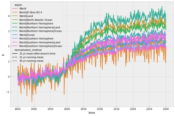
[14]:
ax = plt.figure(figsize=(12, 8)).add_subplot(111)
stitched_normalised_subset = stitched_normalised.filter(
    normalisation_method="*dedrift", keep=False
)
stitched_normalised_subset.lineplot(
    hue="region", style="normalisation_method", ax=ax
);
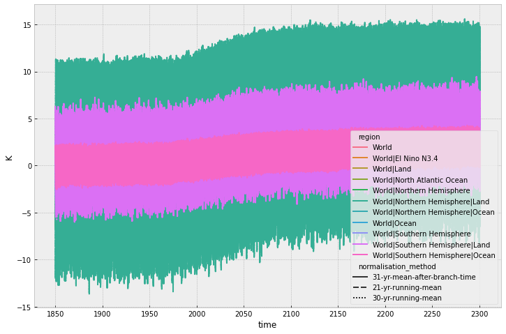
As we have monthly data, this doesn’t tell us much yet. We can take an annual mean before plotting to see a clearer picture.
[15]:
ax = plt.figure(figsize=(12, 8)).add_subplot(111)
stitched_normalised_subset.time_mean("AC").lineplot(
    hue="region", style="normalisation_method", ax=ax
);
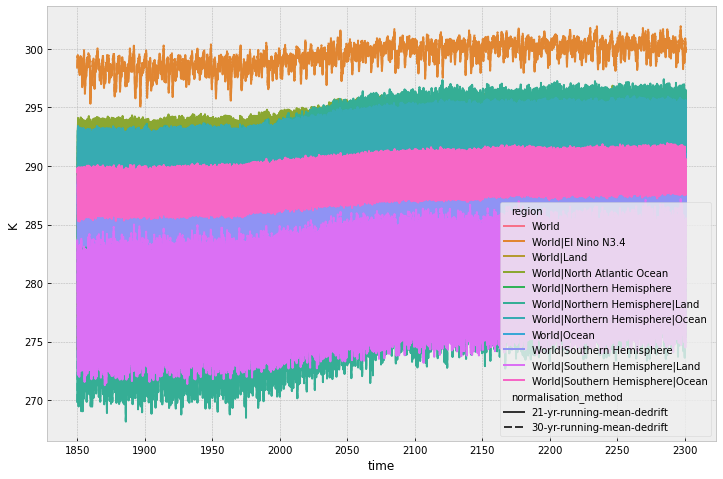
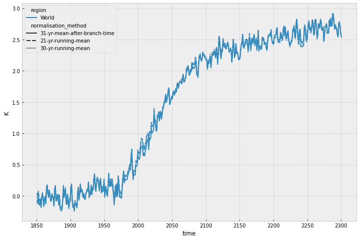
If we only plot world, we get a better sense of the importance of the normalisation method. In this case it makes little difference.
[16]:
ax = plt.figure(figsize=(12, 8)).add_subplot(111)
stitched_normalised_subset.time_mean("AC").filter(region="World").lineplot(
    hue="region", style="normalisation_method", ax=ax
);
With a bit of digging, we can get all the data used to make the above plot.
[17]:
test_cmip5_crunch_output = os.path.join(
    "..",
    "..",
    "..",
    "tests",
    "test-data",
    "expected-crunching-output",
    "marble-cmip5",
    "cmip5",
)
[18]:
# NBVAL_IGNORE_OUTPUT
helper = load_mag_file(
    str(written_files["31-yr-mean-after-branch-time"][0]), drs="MarbleCMIP5"
)


def get_path(generation):
    fp = os.path.join(
        test_cmip5_crunch_output,
        "*",
        helper.metadata["({}) netcdf-scm crunched file".format(generation)],
    )

    return glob.glob(fp)[0]


def load_generation(generation):
    return load_scmrun(get_path(generation))


child = load_generation("child")
parent = load_generation("parent")
normalisation = load_generation("normalisation")

normalisation.head()
[18]:
| time | 0700-01-16 12:00:00 | 0700-02-15 00:00:00 | 0700-03-16 12:00:00 | 0700-04-16 00:00:00 | 0700-05-16 12:00:00 | 0700-06-16 00:00:00 | 0700-07-16 12:00:00 | 0700-08-16 12:00:00 | 0700-09-16 00:00:00 | 0700-10-16 12:00:00 | ... | 1200-03-16 12:00:00 | 1200-04-16 00:00:00 | 1200-05-16 12:00:00 | 1200-06-16 00:00:00 | 1200-07-16 12:00:00 | 1200-08-16 12:00:00 | 1200-09-16 00:00:00 | 1200-10-16 12:00:00 | 1200-11-16 00:00:00 | 1200-12-16 12:00:00 | |||||||||
|---|---|---|---|---|---|---|---|---|---|---|---|---|---|---|---|---|---|---|---|---|---|---|---|---|---|---|---|---|---|---|
| activity_id | climate_model | member_id | mip_era | model | region | scenario | unit | variable | variable_standard_name | |||||||||||||||||||||
| cmip5 | NorESM1-M | r1i1p1 | CMIP5 | unspecified | World|Northern Hemisphere | piControl | K | tas | air_temperature | 280.171925 | 281.224605 | 283.185317 | 286.255835 | 289.475801 | 291.907934 | 292.951130 | 292.815048 | 290.939914 | 287.588672 | ... | 282.980213 | 286.363447 | 289.222116 | 291.663029 | 292.930601 | 292.823846 | 290.665626 | 287.134079 | 283.637265 | 281.104759 |
| World|Southern Hemisphere | piControl | K | tas | air_temperature | 288.463687 | 288.230767 | 287.332330 | 286.383418 | 284.998884 | 283.815010 | 283.269780 | 283.302035 | 284.016765 | 285.182141 | ... | 287.626582 | 286.636466 | 285.385851 | 284.066420 | 283.487844 | 283.684141 | 284.153197 | 285.370605 | 286.527151 | 287.905411 | |||||
| World|Southern Hemisphere|Ocean | piControl | K | tas | air_temperature | 289.557645 | 289.777091 | 289.490769 | 288.722556 | 287.646087 | 286.471247 | 285.760547 | 285.504426 | 286.045069 | 286.766076 | ... | 289.760052 | 288.992076 | 287.921771 | 286.819385 | 286.075362 | 285.941148 | 286.121312 | 286.931792 | 287.909190 | 288.983717 | |||||
| World|North Atlantic Ocean | piControl | K | tas | air_temperature | 289.182025 | 289.093267 | 289.323014 | 290.406649 | 291.320640 | 292.620792 | 293.442007 | 293.952419 | 293.612826 | 292.629936 | ... | 289.903485 | 290.707233 | 291.399045 | 292.689253 | 293.735477 | 294.170233 | 293.738846 | 292.723627 | 291.517845 | 290.198402 | |||||
| World | piControl | K | tas | air_temperature | 284.317806 | 284.727686 | 285.258824 | 286.319627 | 287.237342 | 287.861472 | 288.110455 | 288.058541 | 287.478340 | 286.385407 | ... | 285.303398 | 286.499957 | 287.303983 | 287.864725 | 288.209223 | 288.253993 | 287.409412 | 286.252342 | 285.082208 | 284.505085 |
5 rows × 6012 columns
We can then recover the branching time.
[19]:
branching_time = get_branch_time(parent, parent_path=get_path("normalisation"))
branching_time
[19]:
datetime.datetime(700, 1, 1, 0, 0)
We can then shift our normalisation such that the branch times line up.
[20]:
# NBVAL_IGNORE_OUTPUT
normalisation_shifted = normalisation.timeseries()
normalisation_shifted.columns = normalisation_shifted.columns.map(
    lambda x: dt.datetime(
        x.year - branching_time.year + parent["time"].min().year,
        x.month,
        x.day,
        x.hour,
    )
)
normalisation_shifted = normalisation_shifted.reset_index()
normalisation_shifted["scenario"] = "piControl-shifted"
normalisation_shifted = ScmRun(normalisation_shifted)
normalisation_shifted.head()
[20]:
| time | 1850-01-16 12:00:00 | 1850-02-15 00:00:00 | 1850-03-16 12:00:00 | 1850-04-16 00:00:00 | 1850-05-16 12:00:00 | 1850-06-16 00:00:00 | 1850-07-16 12:00:00 | 1850-08-16 12:00:00 | 1850-09-16 00:00:00 | 1850-10-16 12:00:00 | ... | 2350-03-16 12:00:00 | 2350-04-16 00:00:00 | 2350-05-16 12:00:00 | 2350-06-16 00:00:00 | 2350-07-16 12:00:00 | 2350-08-16 12:00:00 | 2350-09-16 00:00:00 | 2350-10-16 12:00:00 | 2350-11-16 00:00:00 | 2350-12-16 12:00:00 | |||||||||
|---|---|---|---|---|---|---|---|---|---|---|---|---|---|---|---|---|---|---|---|---|---|---|---|---|---|---|---|---|---|---|
| activity_id | climate_model | member_id | mip_era | model | region | scenario | unit | variable | variable_standard_name | |||||||||||||||||||||
| cmip5 | NorESM1-M | r1i1p1 | CMIP5 | unspecified | World|Northern Hemisphere | piControl-shifted | K | tas | air_temperature | 280.171925 | 281.224605 | 283.185317 | 286.255835 | 289.475801 | 291.907934 | 292.951130 | 292.815048 | 290.939914 | 287.588672 | ... | 282.980213 | 286.363447 | 289.222116 | 291.663029 | 292.930601 | 292.823846 | 290.665626 | 287.134079 | 283.637265 | 281.104759 |
| World|Southern Hemisphere | piControl-shifted | K | tas | air_temperature | 288.463687 | 288.230767 | 287.332330 | 286.383418 | 284.998884 | 283.815010 | 283.269780 | 283.302035 | 284.016765 | 285.182141 | ... | 287.626582 | 286.636466 | 285.385851 | 284.066420 | 283.487844 | 283.684141 | 284.153197 | 285.370605 | 286.527151 | 287.905411 | |||||
| World|Southern Hemisphere|Ocean | piControl-shifted | K | tas | air_temperature | 289.557645 | 289.777091 | 289.490769 | 288.722556 | 287.646087 | 286.471247 | 285.760547 | 285.504426 | 286.045069 | 286.766076 | ... | 289.760052 | 288.992076 | 287.921771 | 286.819385 | 286.075362 | 285.941148 | 286.121312 | 286.931792 | 287.909190 | 288.983717 | |||||
| World|North Atlantic Ocean | piControl-shifted | K | tas | air_temperature | 289.182025 | 289.093267 | 289.323014 | 290.406649 | 291.320640 | 292.620792 | 293.442007 | 293.952419 | 293.612826 | 292.629936 | ... | 289.903485 | 290.707233 | 291.399045 | 292.689253 | 293.735477 | 294.170233 | 293.738846 | 292.723627 | 291.517845 | 290.198402 | |||||
| World | piControl-shifted | K | tas | air_temperature | 284.317806 | 284.727686 | 285.258824 | 286.319627 | 287.237342 | 287.861472 | 288.110455 | 288.058541 | 287.478340 | 286.385407 | ... | 285.303398 | 286.499957 | 287.303983 | 287.864725 | 288.209223 | 288.253993 | 287.409412 | 286.252342 | 285.082208 | 284.505085 |
5 rows × 6012 columns
[21]:
# NBVAL_IGNORE_OUTPUT
source_data = run_append([child, parent, normalisation, normalisation_shifted])
source_data.head()
[21]:
| time | 0700-01-16 12:00:00 | 0700-02-15 00:00:00 | 0700-03-16 12:00:00 | 0700-04-16 00:00:00 | 0700-05-16 12:00:00 | 0700-06-16 00:00:00 | 0700-07-16 12:00:00 | 0700-08-16 12:00:00 | 0700-09-16 00:00:00 | 0700-10-16 12:00:00 | ... | 2350-03-16 12:00:00 | 2350-04-16 00:00:00 | 2350-05-16 12:00:00 | 2350-06-16 00:00:00 | 2350-07-16 12:00:00 | 2350-08-16 12:00:00 | 2350-09-16 00:00:00 | 2350-10-16 12:00:00 | 2350-11-16 00:00:00 | 2350-12-16 12:00:00 | |||||||||
|---|---|---|---|---|---|---|---|---|---|---|---|---|---|---|---|---|---|---|---|---|---|---|---|---|---|---|---|---|---|---|
| activity_id | climate_model | member_id | mip_era | model | region | scenario | unit | variable | variable_standard_name | |||||||||||||||||||||
| cmip5 | NorESM1-M | r1i1p1 | CMIP5 | unspecified | World|Northern Hemisphere | rcp45 | K | tas | air_temperature | NaN | NaN | NaN | NaN | NaN | NaN | NaN | NaN | NaN | NaN | ... | NaN | NaN | NaN | NaN | NaN | NaN | NaN | NaN | NaN | NaN |
| World|Southern Hemisphere | rcp45 | K | tas | air_temperature | NaN | NaN | NaN | NaN | NaN | NaN | NaN | NaN | NaN | NaN | ... | NaN | NaN | NaN | NaN | NaN | NaN | NaN | NaN | NaN | NaN | |||||
| World|Southern Hemisphere|Ocean | rcp45 | K | tas | air_temperature | NaN | NaN | NaN | NaN | NaN | NaN | NaN | NaN | NaN | NaN | ... | NaN | NaN | NaN | NaN | NaN | NaN | NaN | NaN | NaN | NaN | |||||
| World|North Atlantic Ocean | rcp45 | K | tas | air_temperature | NaN | NaN | NaN | NaN | NaN | NaN | NaN | NaN | NaN | NaN | ... | NaN | NaN | NaN | NaN | NaN | NaN | NaN | NaN | NaN | NaN | |||||
| World | rcp45 | K | tas | air_temperature | NaN | NaN | NaN | NaN | NaN | NaN | NaN | NaN | NaN | NaN | ... | NaN | NaN | NaN | NaN | NaN | NaN | NaN | NaN | NaN | NaN |
5 rows × 12024 columns
The next cell makes a plot which shows how the 31 year mean after branching time method works.
[22]:
region_to_plot = "World"
norm_method = "31-yr-mean-after-branch-time"
full_view_xlim = [600, 2350]

fig = plt.figure(figsize=(16, 9))


def get_plot_df(src_data):
    out = src_data.time_mean("AC").long_data()
    out["time"] = out["time"].apply(lambda x: x.year)

    return out


ax = fig.add_subplot(311)
sns_df = get_plot_df(
    source_data.filter(scenario="*shifted", keep=False).filter(
        region=region_to_plot,
    )
)
sns.lineplot(
    data=sns_df, x="time", y="value", hue="scenario", style="region", ax=ax
)
ax.axvspan(
    branching_time.year,
    branching_time.year + 31,
    label="normalisation period in raw piControl",
    alpha=0.5,
    color="gray",
)
ax.set_xlim(full_view_xlim)

ax = fig.add_subplot(312)
sns_df = get_plot_df(
    source_data.filter(scenario="piControl", keep=False).filter(
        region=region_to_plot,
    )
)
ax = sns.lineplot(
    data=sns_df, x="time", y="value", hue="scenario", style="region", ax=ax
)

tmp = stitched_normalised.filter(
    region=region_to_plot,
    year=range(1700, 2351),
    normalisation_method=norm_method,
).timeseries()
tmp.index = normalisation.filter(region=region_to_plot).timeseries().index

normaliser = get_normaliser(norm_method)
reference_values = normaliser.get_reference_values(
    pymagicc.io.MAGICCData(tmp),
    normalisation.filter(region=region_to_plot),
    branching_time,
)
ax.plot(
    reference_values.columns.map(lambda x: x.year).values.squeeze(),
    reference_values.values.squeeze(),
    label="normalisation reference values",
    color="lime",
)


ax.axvspan(
    parent["time"].min().year,
    parent["time"].min().year + 31,
    label="normalisation period in shifted piControl\n(same data just different time axis)",
    alpha=0.5,
    color="gray",
)
ax.set_xlim(full_view_xlim)
ax.legend()

ax = fig.add_subplot(313)
sns_df = get_plot_df(
    stitched_normalised.filter(
        region=region_to_plot,
        year=range(1700, 2351),
        normalisation_method=norm_method,
    )
)
sns.lineplot(
    data=sns_df, x="time", y="value", hue="scenario", style="region", ax=ax
)

plt.tight_layout();
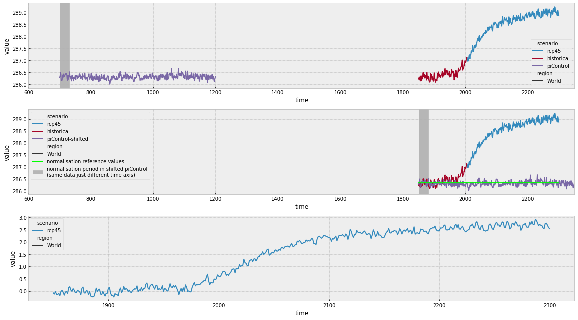
In the top panel above, we can see how the historical and rcp45 simulations have been joined. We can also see the normalisation period that is used. In the middle panel we can see how these compare when the time axes are shifted as well as the values which are used to normalise the simulations. In the bottom panel, we can see the resulting stitched and normalised timeseries.
Next we produce a similar plot for the 21-year (or 30-year) running mean method.
[23]:
region_to_plot = "World"
norm_method = "21-yr-running-mean"
# norm_method = "30-yr-running-mean"
full_view_xlim = [600, 2350]

fig = plt.figure(figsize=(16, 9))


def get_plot_df(src_data):
    out = src_data.time_mean("AC").long_data()
    out["time"] = out["time"].apply(lambda x: x.year)

    return out


ax = fig.add_subplot(311)
sns_df = get_plot_df(
    source_data.filter(scenario="*shifted", keep=False).filter(
        region=region_to_plot,
    )
)
sns.lineplot(
    data=sns_df, x="time", y="value", hue="scenario", style="region", ax=ax
)
ax.axvspan(
    branching_time.year,
    branching_time.year + child["time"].max().year - parent["time"].min().year,
    label="normalisation period in raw piControl",
    alpha=0.5,
    color="gray",
)
ax.set_xlim(full_view_xlim)

for i, (no, xlim) in enumerate(zip((323, 324), ([1000, 2300], [1845, 1880]))):
    ax = fig.add_subplot(no)
    sns_df = get_plot_df(
        source_data.filter(scenario="piControl", keep=False).filter(
            region=region_to_plot, year=range(xlim[0], xlim[1] + 1)
        )
    )
    ax = sns.lineplot(
        data=sns_df, x="time", y="value", hue="scenario", style="region", ax=ax
    )

    tmp = stitched_normalised.filter(
        region=region_to_plot,
        year=range(xlim[0], xlim[1] + 1),
        normalisation_method=norm_method,
    ).timeseries()
    tmp.index = normalisation.filter(region=region_to_plot).timeseries().index

    normaliser = get_normaliser(norm_method)
    reference_values = get_plot_df(
        ScmRun(
            normaliser.get_reference_values(
                pymagicc.io.MAGICCData(tmp),
                normalisation.filter(region=region_to_plot),
                branching_time,
            )
        )
    )
    ax.plot(
        reference_values["time"],
        reference_values["value"],
        label="normalisation reference values",
        color="lime",
    )

    ax.axvspan(
        parent["time"].min().year,
        child["time"].max().year,
        label="normalisation period in shifted piControl\n(same data just different time axis)",
        alpha=0.5,
        color="gray",
    )

    if i == 1:
        ax.get_legend().remove()

    ax.set_xlim(xlim)

ax = fig.add_subplot(313)
sns_df = get_plot_df(
    stitched_normalised.filter(
        region=region_to_plot,
        year=range(1700, 2351),
        normalisation_method=norm_method,
    )
)
sns.lineplot(
    data=sns_df, x="time", y="value", hue="scenario", style="region", ax=ax
)

plt.tight_layout();
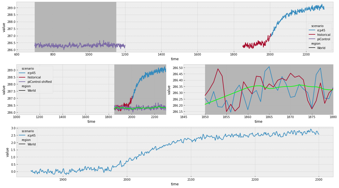
Once again, in the top panel above, we can see how the historical and rcp45 simulations have been joined and the normalisation period that is used. In this case, we use a much longer slice of the piControl run because we need a 21-year running mean over the period corresponding to the scenario runs.
In the middle panels we can see how these compare when the time axes are shifted as well as the values which are used to normalise the simulations (this time with wiggles because it’s a 21-year running mean). The right-hand middle panel illustrates our edge handling. A 21-year running mean can only be taken if there are 21 years around the time point of interest. However, it is often the case that the piControl data starts in the same year as the experiment data. In such a case, to fill in the first 10 years (where a 21 year window is not available), we simply linearly extrapolate the running mean. It would be possible to make other choices, e.g. assuming a constant value or fitting some other curve. However, given how short the time period that must be filled is and how linear CMIP drifts are, other choices will make little difference.
In the bottom panel, we can see the resulting stitched and normalised timeseries.
Plotting function
As a last step, we demonstrate a function which will make plots like the above for a given file. This could be run on lots of files to examine how the normalisation works in batches.
[24]:
def plot_normalisation(
    inpath,
    netcdf_scm_crunched_root_dir,
    region_to_plot,
    axes,
    norm_colour="tab:green",
    dashes=[(10, 5)],
    legend=True,
    drs="MarbleCMIP5",
):
    mag_data = load_mag_file(str(inpath), drs=drs)

    return plot_normalisation_scmdf(
        mag_data.filter(region=region_to_plot),
        netcdf_scm_crunched_root_dir,
        region_to_plot,
        axes,
        norm_colour=norm_colour,
        dashes=dashes,
        legend=legend,
    )


def get_highest_valid_level_and_source_files(
    scmdata, netcdf_scm_crunched_root_dir
):
    source_files = {
        "normalisation": os.path.join(
            netcdf_scm_crunched_root_dir,
            scmdata.metadata["(normalisation) netcdf-scm crunched file"],
        )
    }

    level = "child"
    for i in range(20):
        level_key = "({})".format(level)
        try:
            source_files[level] = os.path.join(
                netcdf_scm_crunched_root_dir,
                scmdata.metadata[
                    "{} netcdf-scm crunched file".format(level_key)
                ],
            )
        except KeyError:
            break

        highest_valid_level = level
        level = (
            step_up_family_tree(level_key).replace("(", "").replace(")", "")
        )
    else:
        raise ValueError("level = {}, really?".format(level))

    return highest_valid_level, source_files


def get_shifted_normalisation(
    normalisation, branching_time, highest_level_start
):
    normalisation_shifted = normalisation.timeseries()

    normalisation_shifted.columns = normalisation_shifted.columns.map(
        lambda x: dt.datetime(
            x.year - branching_time.year + highest_level_start.year,
            x.month,
            x.day,
            x.hour,
        )
    )
    normalisation_shifted = normalisation_shifted.reset_index()
    normalisation_shifted["scenario"] = "{}-shifted".format(
        normalisation.get_unique_meta("scenario", no_duplicates=True)
    )
    normalisation_shifted = ScmRun(normalisation_shifted)

    return normalisation_shifted


def get_plot_df(src_data):
    out = src_data.time_mean("AC").long_data()
    out["time"] = out["time"].apply(lambda x: x.year)

    return out


def make_plot(
    axes,
    source_data,
    source_scmdfs,
    stitched_normalised,
    region_to_plot,
    branching_time,
    highest_level,
    highest_level_start,
    norm_colour,
    dashes,
    legend,
):
    sns_df = get_plot_df(
        source_data.filter(scenario="*shifted", keep=False).filter(
            region=region_to_plot,
        )
    )
    axes[0] = sns.lineplot(
        data=sns_df,
        x="time",
        y="value",
        hue="scenario",
        style="region",
        ax=axes[0],
        dashes=dashes,
        legend=legend if not legend else "brief",
    )
    axes[0].axvline(
        branching_time.year,
        label="branch point in raw piControl",
        alpha=0.5,
        color="gray",
    )
    if legend:
        axes[0].legend()

    axes[0].set_title("Raw data")

    sns_df = get_plot_df(
        source_data.filter(
            scenario=source_scmdfs["normalisation"].get_unique_meta(
                "scenario", no_duplicates=True
            ),
            keep=False,
        ).filter(region=region_to_plot,)
    )

    existing_handles, existing_labels = axes[1].get_legend_handles_labels()

    axes[1] = sns.lineplot(
        data=sns_df,
        x="time",
        y="value",
        hue="scenario",
        style="region",
        ax=axes[1],
        dashes=dashes,
        legend=legend if not legend else "brief",
    )

    tmp = stitched_normalised.filter(region=region_to_plot,).timeseries()
    tmp.index = (
        source_scmdfs["normalisation"]
        .filter(region=region_to_plot)
        .timeseries()
        .index
    )

    normaliser = get_normaliser(
        stitched_normalised.metadata["normalisation method"]
    )
    reference_values = normaliser.get_reference_values(
        pymagicc.io.MAGICCData(tmp),
        source_scmdfs["normalisation"].filter(region=region_to_plot),
        branching_time,
    )
    norm_label = "normalisation reference values"
    norm_handle = axes[1].plot(
        reference_values.columns.map(lambda x: x.year).values.squeeze(),
        reference_values.values.squeeze(),
        label=norm_label,
        color=norm_colour,
        dashes=dashes[0],
    )
    axes[1].set_title("Shifted normalisation data")

    axes[1].axvline(
        highest_level_start.year,
        label="branch point in shifted piControl\n(same data just different time axis)",
        alpha=0.5,
        color="gray",
    )
    axes[1].set_xlim(
        source_scmdfs[highest_level]["year"].min() - 100,
        source_scmdfs["child"]["year"].max() + 200,
    )

    if legend:
        axes[1].legend(loc="right")
    else:
        handles = existing_handles + [norm_handle]
        labels = existing_labels + [norm_label]
        axes[1].legend(handles, labels, loc="right")

    sns_df = get_plot_df(stitched_normalised.filter(region=region_to_plot,))
    axes[2] = sns.lineplot(
        data=sns_df,
        x="time",
        y="value",
        hue="scenario",
        style="region",
        ax=axes[2],
        dashes=dashes,
        legend=legend if not legend else "brief",
    )
    axes[2].set_title("Stiched and normalised data")

    return axes


def plot_normalisation_scmdf(
    scmdf_in,
    netcdf_scm_crunched_root_dir,
    region_to_plot,
    axes,
    norm_colour="tab:green",
    dashes=[(10, 5)],
    legend=True,
):
    scmdf = scmdf_in.filter(region_to_plot)
    assert len(axes) == 3, "Must pass in three axes to plot on"

    (
        highest_valid_level,
        source_files,
    ) = get_highest_valid_level_and_source_files(
        scmdf, netcdf_scm_crunched_root_dir
    )

    source_scmdfs = {
        k: load_scmrun(v) for k, v in tqdm.tqdm(source_files.items())
    }

    highest_level_start = source_scmdfs[highest_valid_level]["time"].min()

    branching_time = get_branch_time(
        source_scmdfs[highest_valid_level],
        parent_path=source_files["normalisation"],
    )

    source_scmdfs["normalisation_shifted"] = get_shifted_normalisation(
        source_scmdfs["normalisation"], branching_time, highest_level_start,
    )

    source_data = run_append([v for v in source_scmdfs.values()])

    return make_plot(
        axes,
        source_data,
        source_scmdfs,
        scmdf_in,
        region_to_plot,
        branching_time,
        highest_valid_level,
        highest_level_start,
        norm_colour,
        dashes,
        legend,
    )
[25]:
# NBVAL_IGNORE_OUTPUT
netcdf_scm_crunched_root_dir = os.path.join(
    "..",
    "..",
    "..",
    "tests",
    "test-data",
    "expected-crunching-output",
    "marble-cmip5",
    "cmip5",
    "Amon",
)
[26]:
# NBVAL_IGNORE_OUTPUT
fig, axes = plt.subplots(nrows=3, ncols=1, figsize=(16, 18))
axes = axes.flatten()

cfgs = {
    "31-yr-mean-after-branch-time": ("tab:green", [(1, 1)]),
    "21-yr-running-mean": ("tab:orange", [(None, None)]),
    "30-yr-running-mean": ("tab:red", [(5, 3)]),
}
for i, (n, f) in enumerate(written_files.items()):
    if n not in cfgs:
        continue

    print(n)
    colour, dashes = cfgs[n]
    plot_normalisation(
        f[0],
        netcdf_scm_crunched_root_dir,
        "World",
        axes,
        norm_colour=colour,
        dashes=dashes,
        legend=True if i == 0 else False,
    )

plt.tight_layout()
0%| | 0/3 [00:00<?, ?it/s]
31-yr-mean-after-branch-time
100%|██████████| 3/3 [00:17<00:00,  5.94s/it]
  0%|          | 0/3 [00:00<?, ?it/s]
21-yr-running-mean
100%|██████████| 3/3 [00:18<00:00,  6.05s/it]
<ipython-input-24-57a3f71751a0>:189: UserWarning: Legend does not support [<matplotlib.lines.Line2D object at 0x16094b610>] instances.
A proxy artist may be used instead.
See: https://matplotlib.org/users/legend_guide.html#creating-artists-specifically-for-adding-to-the-legend-aka-proxy-artists
  axes[1].legend(handles, labels, loc="right")
  0%|          | 0/3 [00:00<?, ?it/s]
30-yr-running-mean
100%|██████████| 3/3 [00:17<00:00,  5.90s/it]
<ipython-input-24-57a3f71751a0>:189: UserWarning: Legend does not support [<matplotlib.lines.Line2D object at 0x162bfc6a0>] instances.
A proxy artist may be used instead.
See: https://matplotlib.org/users/legend_guide.html#creating-artists-specifically-for-adding-to-the-legend-aka-proxy-artists
  axes[1].legend(handles, labels, loc="right")
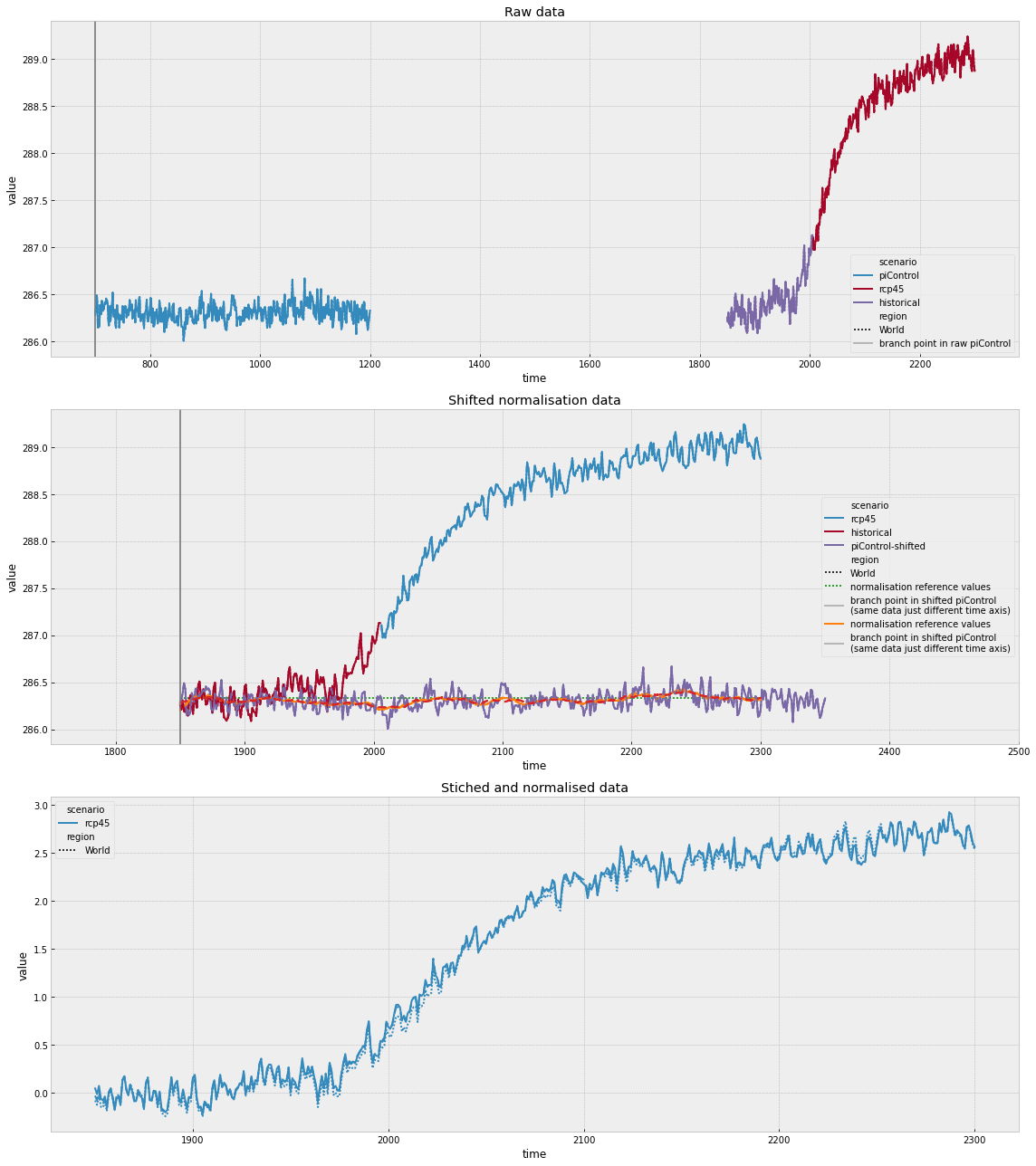
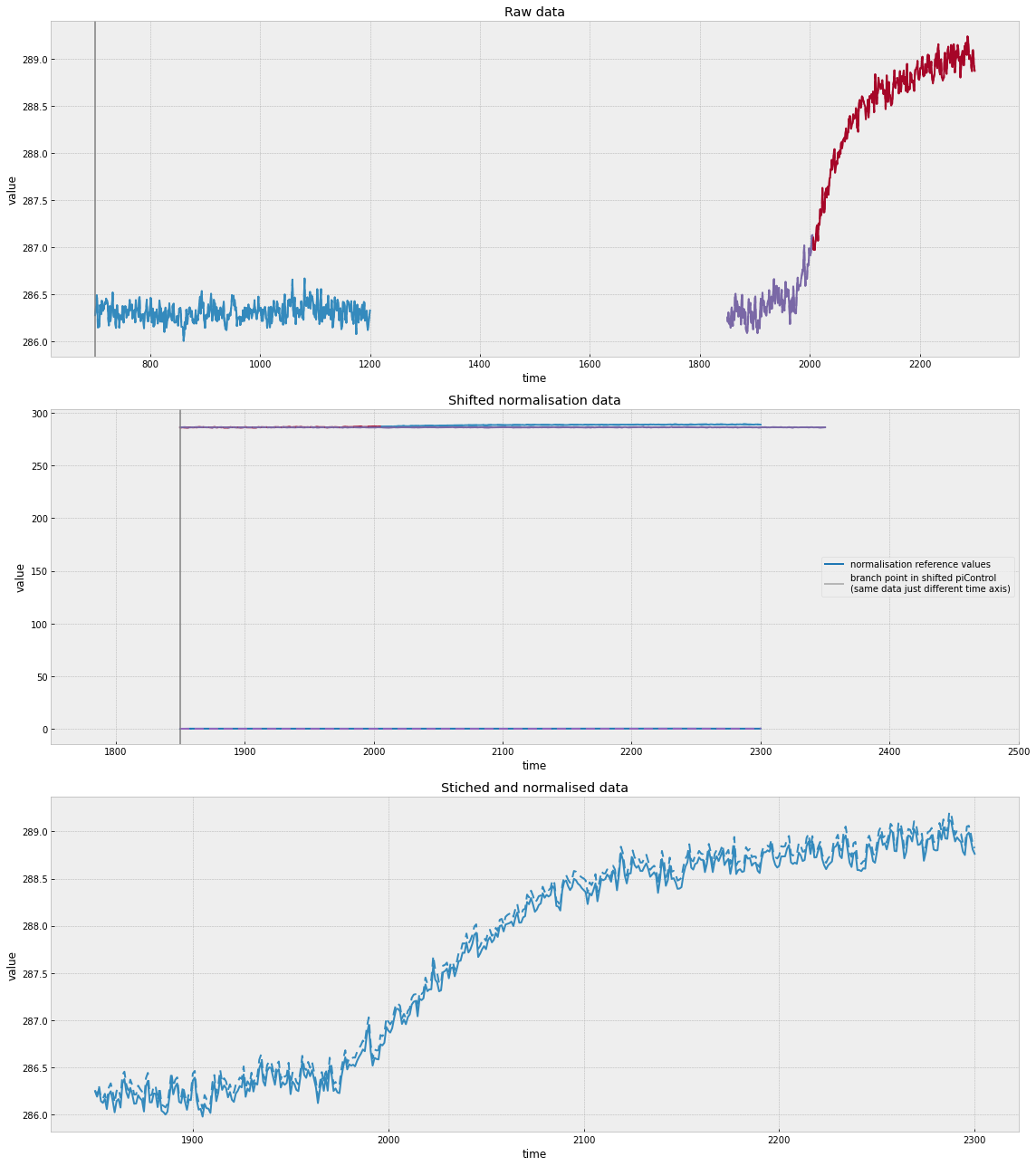
Note that below the normalisation values are intended for drifting, hence are zero, a very different magnitude to the ~287K of the raw data. This is why the middle plot is not exactly illuminating.
[27]:
# NBVAL_IGNORE_OUTPUT
fig, axes = plt.subplots(nrows=3, ncols=1, figsize=(16, 18))
axes = axes.flatten()

cfgs = {
    "21-yr-running-mean-dedrift": ("tab:blue", [(None, None)]),
    "30-yr-running-mean-dedrift": ("tab:purple", [(5, 3)]),
}
for i, (n, f) in enumerate(written_files.items()):
    if n not in cfgs:
        continue

    print(n)
    colour, dashes = cfgs[n]
    plot_normalisation(
        f[0],
        netcdf_scm_crunched_root_dir,
        "World",
        axes,
        norm_colour=colour,
        dashes=dashes,
        legend=True if i == 0 else False,
    )

plt.tight_layout()
0%| | 0/3 [00:00<?, ?it/s]
21-yr-running-mean-dedrift
100%|██████████| 3/3 [00:17<00:00,  5.93s/it]
<ipython-input-24-57a3f71751a0>:189: UserWarning: Legend does not support [<matplotlib.lines.Line2D object at 0x16091b940>] instances.
A proxy artist may be used instead.
See: https://matplotlib.org/users/legend_guide.html#creating-artists-specifically-for-adding-to-the-legend-aka-proxy-artists
  axes[1].legend(handles, labels, loc="right")
  0%|          | 0/3 [00:00<?, ?it/s]
30-yr-running-mean-dedrift
100%|██████████| 3/3 [00:16<00:00,  5.66s/it]
<ipython-input-24-57a3f71751a0>:189: UserWarning: Legend does not support [<matplotlib.lines.Line2D object at 0x162be9610>] instances.
A proxy artist may be used instead.
See: https://matplotlib.org/users/legend_guide.html#creating-artists-specifically-for-adding-to-the-legend-aka-proxy-artists
  axes[1].legend(handles, labels, loc="right")